Last Updated on January 2, 2026
In this tutorial, we’ll build a Microsoft Power BI model that analyzes project profitability by combining accounting, timesheet, employee, and expense data. The model allocates staff and overhead costs across projects to calculate true margins and supports what-if forecasting to test changes in revenue, salaries, or hours.
We’ll go step by step — loading the source data, creating a clean data model, writing key DAX measures, setting up allocation logic, and building a dynamic cost allocation and profitability dashboard you can tailor to your own projects.
By the end, you can preview the dashboard or download the complete package, including the Power BI (.pbix) file, DAX measures, and the data sources used in this tutorial.
Table of Contents
Step 1. Loading Data into Microsoft Power BI
In this first step, we’ll load all project datasets into an empty Microsoft Power BI report, align a few data fields for consistency, and generate a calendar table that will later serve as our time dimension for modeling project costs and profitability.
Step 1a. Importing and Preparing the Data
Go to Power BI’s Home tab, click the Get Data icon, and select the Text/CSV option. In this tutorial we’ll use four datasets:
- accounting_pl – the company’s 2025 accounting profit and loss file with monthly revenue and expense lines.
- employees – employee master data including ID, role, department, and annual employer cost.
- timesheets – weekly time records showing hours worked by project and task.
- expenses – detailed project-related expenses such as travel, meals, and software.
After loading these files into Power BI Desktop, check each table in Data view to confirm data types and column names. This helps ensure smooth joins and prevents type mismatches later when building relationships.
Step 1b. Data Transformation in Power Query
Next, open Transform Data to access the Power Query Editor. In the accounting_pl table, the Date column is stored in a YYYY-MM format, while other datasets use full dates. Convert it into a standard date value (e.g., 2025-01-01) so all tables align by day. Select the Date column and change its Data Type to Date from the Transform tab.
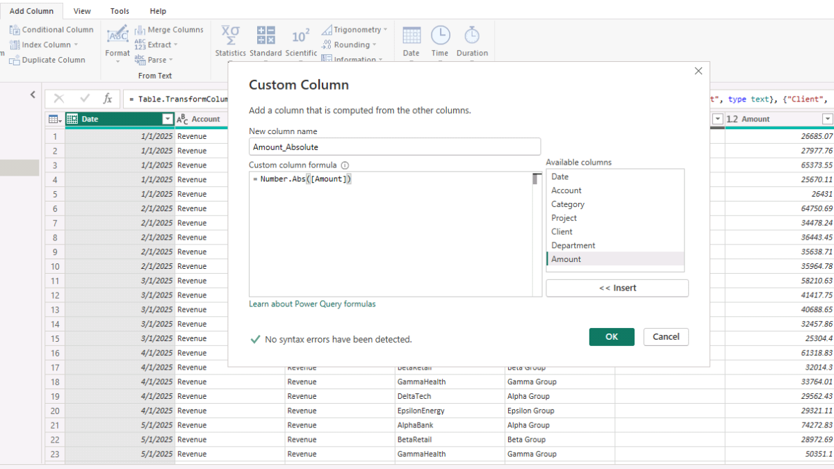
Because the accounting table contains both revenues and expenses, add a helper column with positive numbers only. This simplifies later aggregations where the direction of profit or loss isn’t required. Go to Add Column → Custom Column, enter Number.Abs([Amount]), and name the new field Amount_Absolute. Then set its data type to Decimal Number. When finished, click Close & Apply to load the transformed data back into Power BI.
Step 1c. Creating an Auto-Generated Calendar
A calendar table is essential for accurate time intelligence. It lets Power BI recognize date relationships and simplifies DAX time-based calculations. We’ll create one using DAX rather than importing an external date file.
Table Name: Calendar
Purpose: Generates a continuous date table with fields such as Year, Month, Quarter, and Year-Month Number for consistent period-based analysis across all fact tables.
Calendar =
ADDCOLUMNS (
    CALENDARAUTO(),
    "Year",        YEAR ( [Date] ),
    "MonthNo",     MONTH ( [Date] ),
    "Month",       FORMAT ( [Date], "MMMM" ),
    "Quarter",     "Q" & FORMAT ( [Date], "Q" ),
    "YearMonth",   FORMAT ( [Date], "YYYY-MM" ),
    "YearMonthNum", YEAR([Date]) * 100 + MONTH([Date]),
    "WeekStartMon", [Date] - WEEKDAY ( [Date], 2 ) + 1,
    "MonthStart",   DATE ( YEAR ( [Date] ), MONTH ( [Date] ), 1 ),
    "MonthEnd",     EOMONTH ( [Date], 0 )
)
In Model view, select Table tools → New table, paste the DAX above, and press Enter. The Calendar table will later connect to the accounting, expenses, and timesheets data, ensuring all analyses share a common date hierarchy.
With the datasets loaded, transformed, and the calendar table ready, we can move on to next step, where we’ll create relationships and finalize the Power BI data model that underpins our allocation analysis.
Step 2. Table Relationships and Data Model in Microsoft Power BI
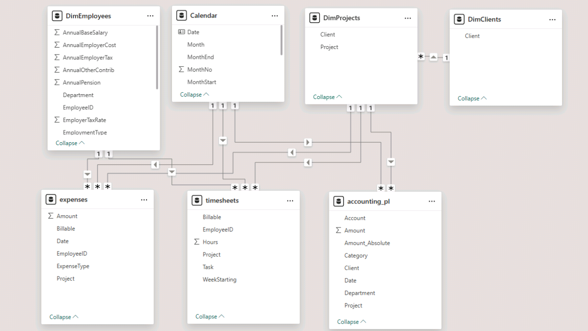
In this step, we’ll shape a clean star schema with dimensions (Calendar, Employees, Clients, Projects) on top and fact tables (accounting_pl, expenses, timesheets) below. Using Model view in Power BI Desktop, we’ll connect these tables and prepare the foundation for all later calculations.
Step 2a. Arrange the model and connect facts to dimensions
Open Model view (the left sidebar icon showing the table diagram). Each table appears as a rectangular card listing its columns. Arrange the layout with dimensions at the top and fact tables below.
First, connect DimEmployees[EmployeeID] to expenses[EmployeeID] and timesheets[EmployeeID]. When prompted, set the relationship to one-to-many, active, and use a single cross-filter direction (from DimEmployees to the facts).
Next, link Calendar[Date] to accounting_pl[Date] and expenses[Date]. For the timesheets table, use Calendar[Date] → timesheets[WeekStarting], since this column defines the time period for recorded hours. These one-to-many relationships ensure filters flow consistently from dimensions to facts.
Step 2b. Create project and client dimensions with DAX
To make the model easier to filter and navigate, add two lightweight DAX tables.
DimProjects – unique Project–Client combinations derived from the accounting data. Used to group or filter results at the project level.
DimProjects =
DISTINCT (
    SELECTCOLUMNS (
        accounting_pl,
        "Project", accounting_pl[Project],
        "Client",  accounting_pl[Client]
    )
)
DimClients – unique Client list for high-level filtering and for driving the client–project hierarchy.
DimClients =
DISTINCT ( SELECTCOLUMNS ( accounting_pl, "Client", accounting_pl[Client] ) )
After creating these tables, set the following relationships:
- DimClients[Client] → DimProjects[Client] – one-to-many, single direction (clients filter projects).
- DimProjects[Project] → accounting_pl[Project], expenses[Project], timesheets[Project] – one-to-many, single direction (projects filter facts).
Finally, rename employees to DimEmployees (right-click the table in Model view and choose Rename) to stay consistent with naming conventions.
Step 2c. Modeling tip: control automatic relationship detection
For a cleaner model, open File › Options and settings › Options › Current File › Data Load, and uncheck “Autodetect new relationships after data is loaded.” This ensures relationships are only created intentionally, avoiding unexpected joins that can complicate your Power BI model.
With the model structure finalized and relationships defined, we’re ready to create the first set of DAX measures that will calculate revenues, costs, and hours across projects.
Step 3. Baseline Project Metrics in Microsoft Power BI
We’ll build a compact baseline report that aggregates revenue, direct expenses, and hours across projects. To keep everything organized, create a dedicated Measures_Table (Report view → Enter data → name it Measures_Table; no rows needed) and add the core measures below—each with a short purpose statement for this tutorial.
Step 3a. Core DAX measures (with purpose)
Total Revenue — sums recognized revenue from the accounting P&L to establish the top line for each period and project.
Total Revenue =
CALCULATE (
    SUM ( accounting_pl[Amount_Absolute] ),
    accounting_pl[Category] = "Revenue"
)
Total Direct Expenses — aggregates project-level outlays from the expenses table (e.g., travel, software, training) used directly in delivery.
Total Direct Expenses =
SUM ( expenses[Amount] )
Total Non-Direct Cost — captures non-direct costs from the P&L (rent, utilities, overheads) after removing direct project expenses; this forms the pool we’ll allocate later.
Total Non-Direct Cost =
VAR PLCostsOnly =
    CALCULATE (
        SUM ( accounting_pl[Amount_Absolute] ),
        accounting_pl[Category] <> "Revenue"
    )
RETURN PLCostsOnly - [Total Direct Expenses]
Total Hours — total effort logged on projects, used for utilization and hour-based allocation.
Total Hours =
SUM ( timesheets[Hours] )
Billable Hours — subset of effort marked billable, used later for billing-rate and margin-per-hour analysis.
Billable Hours =
CALCULATE ( [Total Hours], timesheets[Billable] = "Y" )
Step 3b. Build a baseline matrix and add slicers
In Report view, insert a Matrix visual. Place Calendar[MonthStart] on Rows, and add Total Revenue, Total Direct Expenses, Total Non-Direct Cost, and Total Hours to Values. Format the first three as currency and Total Hours as a whole number.
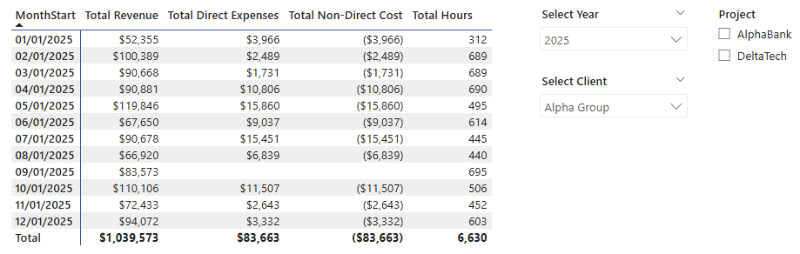
Add three slicers to make the view interactive: Calendar[Year] (Dropdown), DimClients[Client] (Dropdown), and DimProjects[Project] (Dropdown or Vertical list). The Project slicer’s options will respond to the selected Client, and the matrix will update accordingly—confirming that the relationships from dimensions to facts are working as designed.
Step 4. DAX Measures for Cost Allocation
Direct expenses tell only part of the story. To understand true project margins, we’ll (a) assign staff costs to projects using timesheets and employee rates, and (b) allocate non-direct costs (overheads and unallocated salaries) by a chosen basis — Hours or Revenue.
Step 4a. Employee cost allocation
We’ll calculate a fully loaded hourly cost for each employee (based on annual employer cost and contracted weekly hours) and multiply it by the hours they spent on each project. This yields the allocated salary cost at the project level.
Allocated Employee Cost (Fully Loaded) — multiplies each employee’s effective hourly rate by their recorded hours on the project to attribute salary cost to delivery.
Allocated Employee Cost (Fully Loaded) =
SUMX (
    timesheets,
    VAR Annual  = RELATED ( DimEmployees[AnnualEmployerCost] )
    VAR Weekly  = COALESCE ( RELATED ( DimEmployees[WeeklyHours] ), 40 )
    VAR HoursYr = Weekly * 52
    VAR Hourly  = DIVIDE ( Annual, HoursYr )
    RETURN timesheets[Hours] * Hourly
)
Step 4b. Allocate non-direct costs by Hours or Revenue
We’ll give the user a simple switch to choose the allocation basis, then compute each project’s share and apply it to the overhead pool.
Allocation Basis — small helper DAX table to drive the slicer (Hours or Revenue). Create it by adding a New Table from the Report View’s Modeling tab.
Allocation Basis =
DATATABLE ( "Basis", STRING, { { "Hours" }, { "Revenue" } } )
Now, add the following DAX measures.
Selected Basis — reads the slicer; defaults to “Hours.”
Selected Basis =
SELECTEDVALUE ( 'Allocation Basis'[Basis], "Hours" )
Hours Share (Projects) — project’s proportion of total hours (excluding “Other”) within current filters.
Hours Share (Projects) =
VAR Num =
    CALCULATE (
        [Total Hours],
        KEEPFILTERS ( DimProjects[Project] <> "Other" )
    )
VAR Den =
    CALCULATE (
        [Total Hours],
        REMOVEFILTERS ( DimProjects[Project] ),
        REMOVEFILTERS ( DimClients[Client] ),
        KEEPFILTERS ( DimProjects[Project] <> "Other" )
    )
RETURN DIVIDE ( Num, Den )
Revenue Share (Projects) — project’s proportion of total recognized revenue (excluding “Other”) within current filters.
Revenue Share (Projects) =
VAR Num =
    CALCULATE (
        [Total Revenue],
        KEEPFILTERS ( DimProjects[Project] <> "Other" )
    )
VAR Den =
    CALCULATE (
        [Total Revenue],
        REMOVEFILTERS ( DimProjects[Project] ),
        REMOVEFILTERS ( DimClients[Client] ),
        KEEPFILTERS ( DimProjects[Project] <> "Other" )
    )
RETURN DIVIDE ( Num, Den )
Allocation Share — switches between hours-based and revenue-based shares per the slicer.
Allocation Share =
VAR b = UPPER ( TRIM ( SELECTEDVALUE ( 'Allocation Basis'[Basis], "HOURS" ) ) )
RETURN IF ( b = "REVENUE", [Revenue Share (Projects)], [Hours Share (Projects)] )
Total Salaries (P&L) — total salaries from the accounting P&L (forms part of the overhead pool).
Total Salaries (P&L) =
CALCULATE (
    SUM ( accounting_pl[Amount_Absolute] ),
    accounting_pl[Account] = "Salaries"
)
Other Non-Direct Cost — non-direct costs excluding salaries; will be allocated along with any unallocated salaries.
Other Non-Direct Cost =
[Total Non-Direct Cost] - [Total Salaries (P&L)]
Unallocated Salaries — the portion of salaries not assigned via timesheets (i.e., outside direct project work).
Unallocated Salaries =
VAR p_salaries = [Total Salaries (P&L)]
VAR allocated  = [Allocated Employee Cost (Fully Loaded)]
RETURN MAX ( 0, p_salaries - allocated )
Total Direct Expenses (filtered for allocation scenarios) — sums direct expenses and excludes the “Other” bucket to keep allocations clean. Note: update this measure in your file to avoid confusion with the version from Step 3.
Total Direct Expenses =
CALCULATE (
    SUM ( expenses[Amount] ),
    KEEPFILTERS ( expenses[Project] <> "Other" )
)
Overhead Pool — global pool of non-direct costs (including any unallocated salaries), evaluated without project or client filters.
Overhead Pool =
VAR PoolGlobal =
    CALCULATE (
        [Total Non-Direct Cost] - [Allocated Employee Cost (Fully Loaded)],
        REMOVEFILTERS ( DimProjects[Project] ),
        REMOVEFILTERS ( DimClients[Client] )
    )
RETURN PoolGlobal
Allocated Overheads — applies the selected allocation share to distribute the overhead pool across projects, skipping the “Other” bucket.
Allocated Overheads =
VAR Pool =
    CALCULATE ( [Overhead Pool], REMOVEFILTERS ( DimProjects[Project] ) )
RETURN
IF (
    SELECTEDVALUE ( DimProjects[Project] ) = "Other",
    BLANK (),
    Pool * [Allocation Share]
)
With staff cost assignment and overhead allocation in place, the model can now calculate fully loaded project costs. Next, we’ll use these measures to visualize project profitability inside a Power BI dashboard.
Step 5. Project Costs and Profitability Power BI Dashboard
With staff and overhead allocations in place, bring everything together in a compact project profit and loss view. We’ll build a monthly matrix, duplicate it for a project view, and add a slicer to switch the allocation basis.
Step 5a. Build the monthly and project P&L
In Report view, insert a Matrix and place Calendar[MonthStart] on Rows. Add Total Revenue, Total Direct Expenses, Allocated Employee Cost (Fully Loaded), and Allocated Overheads to Values. Use Rename for this visual to keep column headers concise. Optionally add Billable Hours for context.
Total Allocated Cost — combines employee cost, direct expenses, and allocated overheads to show the fully loaded delivery cost.
Total Allocated Cost =
[Allocated Employee Cost] + [Total Direct Expenses] + [Allocated Overheads]
Project Profit — revenue minus fully loaded cost for the selected grain (month or project).
Project Profit =
[Total Revenue] - [Total Allocated Cost]
Duplicate the matrix to create a by-project view: replace Calendar[MonthStart] with DimProjects[Project] on Rows.

Step 5b. Add the Allocation Basis slicer
Insert a Slicer and use Allocation Basis[Basis] with Dropdown style.
- Hours (default) allocates overheads and unallocated salaries by each project’s share of total hours.
- Revenue allocates by each project’s share of recognized revenue.
The matrices will update immediately when you switch the basis, confirming the allocation logic is applied end to end.
Step 5c. Project Cost Allocation Check and Reconciliation
Add a simple check to ensure allocated totals match the original P&L.
Total Cost (P&L) — all non-revenue lines from accounting (the ground truth for total costs).
Total Cost (P&L) =
CALCULATE (
    SUM ( accounting_pl[Amount_Absolute] ),
    accounting_pl[Account] <> "Revenue"
)
Allocation Variance — difference between Total Allocated Cost and Total Cost (P&L); should be 0.00 when balanced.
Allocation Variance =
ROUND([Total Allocated Cost] - [Total Cost (P&L)], 2)
Insert a Multi-row card with Total Allocated Cost, Total Cost (P&L), and Allocation Variance. To prevent user filters from affecting the check, open Format › Edit interactions and set slicers/matrices to None for this visual. Matching totals and a zero variance confirm that your allocation is fully reconciled.
Step 6. Timesheets and Staff Project Cost Analysis
Now that we have project-level allocations and profitability measures in place, let’s take a closer look at how much time each employee contributes to projects and what impact that has on revenue and costs. Using the timesheets dataset, we’ll analyze both total and billable hours, calculate employee-level revenue contribution, and assess cost per hour.
By combining this data with the accounting P&L and allocation measures, we can build an employee utilization dashboard that shows each staff member’s share of hours, generated revenue, and gross margin per hour.
To get started, go to the Report View in Microsoft Power BI and select New Table from the Modeling tab. The following DAX creates a simple table where users can toggle between analyzing either billable hours only or all hours recorded in the timesheets.
Hour Basis =
DATATABLE ( "Basis", STRING, { { "Billable Hours" }, { "Total Hours" } } )
Once created, insert a Slicer visual from the Insert tab. Add the field Hour Basis[Basis], set it to Dropdown, and turn on Single Select in the Slicer Settings. This will let users easily switch between total and billable views for all related calculations.
Step 6a. Calculating Employee Shares and Revenue Contribution
We’ll now define DAX measures that calculate each employee’s share of hours within a project and the corresponding portion of revenue. These measures form the foundation for the employee performance dashboard.
Selected Hour Basis – stores the slicer selection (“Billable Hours” or “Total Hours”) to drive later measures dynamically.
Selected Hour Basis =
UPPER ( TRIM ( SELECTEDVALUE ( 'Hour Basis'[Basis], "BILLABLE HOURS" ) ) )
Employee Hours for Share – calculates the number of hours an employee spent on a given project, depending on the hour basis selected.
Employee Hours for Share =
VAR UseBillable = [Selected Hour Basis] = "BILLABLE HOURS"
RETURN
IF (
    UseBillable,
    CALCULATE ( [Billable Hours], KEEPFILTERS ( DimProjects[Project] <> "Other" ) ),
    CALCULATE ( [Total Hours],   KEEPFILTERS ( DimProjects[Project] <> "Other" ) )
)
Project Hours for Share – computes the total number of project hours across all employees, again using the selected hour type.
Project Hours for Share =
VAR UseBillable = [Selected Hour Basis] = "BILLABLE HOURS"
RETURN
IF (
    UseBillable,
    CALCULATE (
        [Billable Hours],
        REMOVEFILTERS ( DimEmployees[EmployeeID] ),
        KEEPFILTERS ( DimProjects[Project] <> "Other" )
    ),
    CALCULATE (
        [Total Hours],
        REMOVEFILTERS ( DimEmployees[EmployeeID] ),
        KEEPFILTERS ( DimProjects[Project] <> "Other" )
    )
)
Employee Share of Project Hours – calculates what portion of total project hours each employee contributed.
Employee Share of Project Hours =
VAR EmpHrsThisProj =
    CALCULATE ( [Total Hours], KEEPFILTERS ( DimProjects[Project] <> "Other" ) )
VAR ProjHrsAllEmps =
    CALCULATE (
        [Total Hours],
        REMOVEFILTERS ( DimEmployees[EmployeeID] ),
        KEEPFILTERS ( DimProjects[Project] <> "Other" )
    )
RETURN DIVIDE ( EmpHrsThisProj, ProjHrsAllEmps )
Employee Revenue Contribution – assigns revenue to each employee proportionally to their share of project hours.
Employee Revenue Contribution =
SUMX (
    FILTER ( VALUES ( DimProjects[Project] ), DimProjects[Project] <> "Other" ),
    VAR EmpHrs = [Employee Hours for Share]
    VAR ProjHrs = [Project Hours for Share]
    VAR ProjRev = CALCULATE ( [Total Revenue] )
    RETURN DIVIDE ( EmpHrs, ProjHrs ) * ProjRev
)
With these measures in place, we can now visualize how each employee contributes to project revenue both in total and on a per-hour basis.
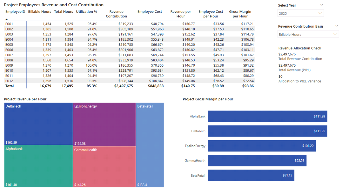
Step 6b. Average Project Revenue and Cost Contribution per Hour
To deepen the analysis, we’ll calculate average revenue, cost, and margin per hour for each employee. Create a Matrix visual in a new report page and add DimEmployees[EmployeeID] to the Rows. Use the measures below to populate the values.
Total Hours (Direct Projects) – sums hours spent on all projects except “Other”.
Total Hours (Direct Projects) =
CALCULATE ( [Total Hours], KEEPFILTERS ( DimProjects[Project] <> "Other" ) )
Billable Hours (Direct Projects) – same as above, limited to billable time.
Billable Hours (Direct Projects) =
CALCULATE ( [Billable Hours], KEEPFILTERS ( DimProjects[Project] <> "Other" ) )
Project Utilization % – calculates how efficiently an employee’s hours are billed versus total hours.
Project Utilization % =
DIVIDE ( [Billable Hours (Direct Projects)], [Total Hours (Direct Projects)] )
Hours Denominator (by Slicer) – adjusts calculations dynamically depending on whether “Billable” or “Total Hours” is selected.
Hours Denominator (by Slicer) =
IF (
    [Selected Hour Basis] = "BILLABLE HOURS",
    [Billable Hours (Direct Projects)],
    [Total Hours (Direct Projects)]
)
Revenue per Hour (Employee) – computes the average hourly revenue contribution for each employee.
Revenue per Hour (Employee) =
DIVIDE ( [Employee Revenue Contribution], [Hours Denominator (by Slicer)] )
Staff Hourly Cost (Fully Loaded) – represents each employee’s average cost per hour, including salary and overheads.
Staff Hourly Cost (Fully Loaded) =
DIVIDE(
    [Allocated Employee Cost (Fully Loaded)],
    [Hours Denominator (by Slicer)]
)
Gross Margin per Hour – the difference between hourly revenue and hourly cost, a key indicator of profitability per employee.
Gross Margin per Hour =
[Revenue per Hour (Employee)] - [Staff Hourly Cost (Fully Loaded)]
After adding the measures, rename columns directly in the visual for readability.
You can extend this analysis further by inserting additional visuals: a Treemap with DimProjects[Project] as Category and Revenue per Hour (Employee) as Value, and a Clustered Bar Chart with DimProjects[Project] on the Y-axis and Gross Margin per Hour on the X-axis.
Because all measures are connected to the same data model, selecting an employee or project filters the entire dashboard, allowing for a seamless analysis of productivity, revenue, and cost efficiency.
Step 7. Parameters and Forecast Measures in Microsoft Power BI
Add what-if parameters to test sensitivities across revenue, direct expenses, salaries, hours, and overheads. These drive simple multipliers that produce a parallel Forecast branch of measures, so you can compare Actuals vs Forecast without touching the base logic.
Step 7a. Adding a Parameter in Microsoft Power BI
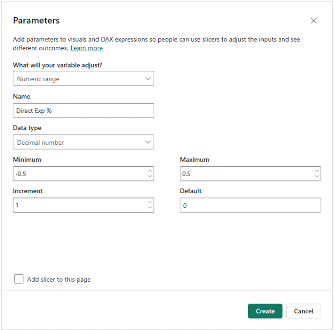
In Power BI Desktop (Modeling → New parameter), create five Numeric Range parameters using Decimal type. I enclosed suggested settings in the brackets but feel free to adjust them to your requirements:
- Revenue % (min −0.50, max +0.50, increment 0.01, default 0)
- Direct Exp % (min −0.50, max +0.50, increment 0.01, default 0)
- Salaries % (min −0.50, max +0.50, increment 0.01, default 0)
- Hours % (min −0.50, max +0.50, increment 0.01, default 0)
- Overhead % (min −0.50, max +0.50, increment 0.01, default 0)
Now add the multipliers, which will be used in the corresponding projections:
Forecast Multipliers — scale actual values for forecast calculations.
Revenue Multiplier = 1 + 'Revenue %'[Revenue % Value]
DirectExp Multiplier = 1 + 'Direct Exp %'[Direct Exp % Value]
Salaries Multiplier  = 1 + 'Salaries %'[Salaries % Value]
Hours Multiplier = 1 + 'Hours %'[Hours % Value]
Overhead Multiplier = 1 + 'Overhead %'[Overhead % Value]
Tip: In Model view, use Display folder in the Properties pane to group “Actuals” vs “Forecast” for easier navigation.
Step 7b. Project Allocation Forecast DAX Measures
Create the forecasted base metrics first, then mirror the allocation logic so Actuals and Forecast can be compared independently.
Total Hours (Forecast) — applies Hours Multiplier to base hours.
Total Hours (Forecast) =
[Total Hours] * [Hours Multiplier]
Billable Hours (Forecast) — billable portion after the Hours Multiplier.
Billable Hours (Forecast) =
[Billable Hours] * [Hours Multiplier]
Utilization % (Forecast) — billable share of forecast hours.
Utilization % (Forecast) =
DIVIDE ( [Billable Hours (Forecast)], [Total Hours (Forecast)] )
Total Revenue (Forecast) — revenue after applying the Revenue Multiplier.
Total Revenue (Forecast) =
[Total Revenue] * [Revenue Multiplier]
Total Direct Expenses (Forecast) — direct expenses after the Direct Exp % assumption.
Total Direct Expenses (Forecast) =
[Total Direct Expenses] * [DirectExp Multiplier]
Total Salaries (P&L) (Forecast) — P&L salaries scaled by the Salaries % assumption.
Total Salaries (P&L) (Forecast) =
[Total Salaries (P&L)] * [Salaries Multiplier]
Unallocated Salaries (Forecast) — unassigned salary portion after Salaries %.
Unallocated Salaries (Forecast) =
[Unallocated Salaries] * [Salaries Multiplier]
Other Non-Direct Cost (Forecast) — non-salary overheads scaled by Overhead %.
Other Non-Direct Cost (Forecast) =
[Other Non-Direct Cost] * [Overhead Multiplier]
Total Non-Direct Cost (Forecast) — recombines salary and other overheads.
Total Non-Direct Cost (Forecast) =
[Other Non-Direct Cost (Forecast)] + [Total Salaries (P&L) (Forecast)]
Allocated Employee Cost (Fully Loaded) (Forecast) — staff cost adjusted by Salaries % and Hours %.
Allocated Employee Cost (Fully Loaded) (Forecast) =
[Allocated Employee Cost (Fully Loaded)]
    * [Salaries Multiplier]
    * [Hours Multiplier]
Hours Share (Projects) (Forecast) — project share of total forecast hours (excluding “Other”).
Hours Share (Projects) (Forecast) =
VAR Num =
    CALCULATE (
        [Total Hours (Forecast)],
        KEEPFILTERS ( DimProjects[Project] <> "Other" )
    )
VAR Den =
    CALCULATE (
        [Total Hours (Forecast)],
        REMOVEFILTERS ( DimProjects[Project] ),
        REMOVEFILTERS ( DimClients[Client] ),
        KEEPFILTERS ( DimProjects[Project] <> "Other" )
    )
RETURN DIVIDE ( Num, Den )
Revenue Share (Projects) (Forecast) — project share of total forecast revenue (excluding “Other”).
Revenue Share (Projects) (Forecast) =
VAR Num =
    CALCULATE (
        [Total Revenue (Forecast)],
        KEEPFILTERS ( DimProjects[Project] <> "Other" )
    )
VAR Den =
    CALCULATE (
        [Total Revenue (Forecast)],
        REMOVEFILTERS ( DimProjects[Project] ),
        REMOVEFILTERS ( DimClients[Client] ),
        KEEPFILTERS ( DimProjects[Project] <> "Other" )
    )
RETURN DIVIDE ( Num, Den )
Allocation Share (Forecast) — switches between forecast Hours/Revenue shares.
Allocation Share (Forecast) =
VAR b = UPPER ( TRIM ( SELECTEDVALUE ( 'Allocation Basis'[Basis], "HOURS" ) ) )
RETURN IF ( b = "REVENUE", [Revenue Share (Projects) (Forecast)], [Hours Share (Projects) (Forecast)] )
Overhead Pool (Forecast) — global pool of forecast non-directs + unallocated salaries (ignores project/client filters).
Overhead Pool (Forecast) =
CALCULATE (
    [Other Non-Direct Cost (Forecast)] + [Unallocated Salaries (Forecast)],
    REMOVEFILTERS ( DimProjects[Project] ),
    REMOVEFILTERS ( DimClients[Client] )
)
Allocated Overheads (Forecast) — distributes the forecast overhead pool; hides for “Other.”
Allocated Overheads (Forecast) =
VAR Pool = [Overhead Pool (Forecast)]
RETURN
IF (
    SELECTEDVALUE ( DimProjects[Project] ) = "Other",
    BLANK (),
    Pool * [Allocation Share (Forecast)]
)
Total Cost (Forecast) — fully loaded forecast cost.
Total Cost (Forecast) =
[Allocated Employee Cost (Fully Loaded) (Forecast)]
    + [Total Direct Expenses (Forecast)]
    + [Allocated Overheads (Forecast)]
Project Profit (Forecast) — forecast margin at the current grain.
Project Profit (Forecast) =
[Total Revenue (Forecast)] - [Total Allocated Cost (Forecast)]
With these measures in place, you can assemble a Forecast dashboard, add parameter slicers, and compare Actuals vs Forecast throughout the model.
Step 8. Project Cost Allocation Forecast and Sensitivity Analysis
With the forecast branch of measures in place, let’s turn them into an interactive forecast dashboard. We’ll start by summarizing project-level results in a matrix, add parameter slicers to test assumptions, then compare Actual vs Forecast using a variance visual. Finally, we’ll surface KPI cards to track per-hour economics.
Step 8a. Build the Forecast Matrix and Parameter Slicers
In Report view, insert a Matrix and place DimProjects[Project] on Rows. Add these measures to Values: Total Revenue (Forecast), Total Direct Expenses (Forecast), Allocated Employee Cost (Fully Loaded) (Forecast), Allocated Overheads (Forecast), Total Allocated Cost (Forecast), and Project Profit (Forecast). Use Rename for this visual to keep column labels concise.
Next, add two Dropdown slicers for context filters: Allocation Basis[Basis] and Calendar[Year]. With all parameters at 0, the forecast mirrors Actuals—this is expected and provides a clean baseline.
To activate sensitivity testing, insert five parameter slicers (Dropdown, Single value, Slider = On): Revenue %, Salaries %, Hours %, Direct Exp %, and Overhead %. Format each as Percent. As you change values (e.g., set Revenue % to 10%), the matrix should immediately reflect the new totals across projects.
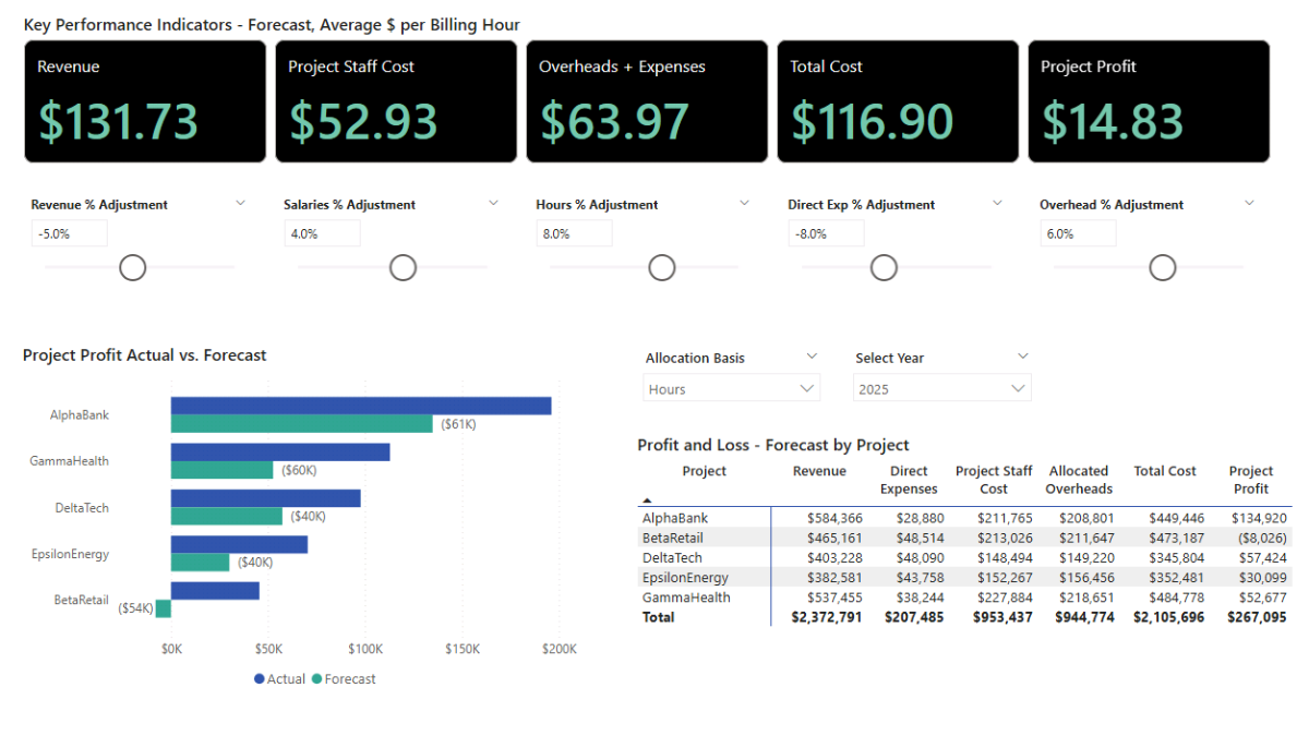
Step 8b. Actual vs Forecast Variance Chart
To visualize how forecast assumptions affect profitability, add a Clustered Bar Chart. Set DimProjects[Project] on the Y-axis and place both Project Profit and Project Profit (Forecast) on the X-axis. Right-click the legend or series names and use Rename for this visual to label them clearly as Actual and Forecast.
Now add a variance label that quantifies the difference between Actual and Forecast:
Project Profit Variance (Actual vs Forecast) =
[Project Profit] - [Project Profit (Forecast)]
Open Format → Data labels. Set Apply settings to the Forecast series, switch on Show for this series, then enable Value and assign Project Profit Variance (Actual vs Forecast) as the field. You’ll now see an intuitive variance overlay directly on the bars.
Step 8c. KPI Cards for Per-Hour Economics
Finally, add Card (new) visuals to surface forecast KPIs that depend on billable hours. These cards help stakeholders interpret how assumptions roll up to revenue and margin efficiency:
Average Billing Rate (Forecast) — forecast revenue per billable hour.
Average Billing Rate (Forecast) =
DIVIDE ( [Total Revenue (Forecast)], [Billable Hours (Forecast)] )
Project Staff Cost per Hour (Forecast) — forecast staff cost per billable hour.
Project Staff Cost per Hour (Forecast) =
[Allocated Employee Cost (Fully Loaded) (Forecast)] / [Billable Hours (Forecast)]
Allocated Overheads + Expenses per Hour (Forecast) — overheads plus direct expenses per billable hour.
Allocated Overheads + Expenses per Hour (Forecast) =
( [Allocated Overheads (Forecast)] + [Total Direct Expenses (Forecast)] ) / [Billable Hours (Forecast)]
Total Cost per Hour (Forecast) — fully loaded cost per billable hour.
Total Cost per Hour (Forecast) =
[Total Cost (Forecast)] / [Billable Hours (Forecast)]
Project Profit per Hour (Forecast) — profit per billable hour.
Project Profit per Hour (Forecast) =
[Project Profit (Forecast)] / [Billable Hours (Forecast)]
Use the Format pane to tidy titles and units. As you adjust parameter sliders, the forecast matrix, variance bars, and KPI cards will all update together—making it easy to explore “what-if” scenarios and communicate how changes in revenue, staffing, hours, or overheads affect project profitability.
📌 Recap: Building a Project Cost Allocation & Forecast Model in Microsoft Power BI
Here’s a quick recap of the steps we followed to build a complete project cost allocation and profitability forecast model in Microsoft Power BI:
- Load and prepare data. Import accounting_pl, employees, timesheets, and expenses; use Power Query for minor fixes (e.g., absolute amounts), and generate a DAX Calendar table.
- Create relationships and a clean star schema. Arrange dimensions (Calendar, DimEmployees, DimClients, DimProjects) above facts and set one-to-many, single-direction relationships.
- Build baseline DAX measures. Define Total Revenue, Total Direct Expenses, Total Non-Direct Cost, Total Hours, and Billable Hours; assemble a baseline matrix with Year/Client/Project slicers.
- Add cost allocation logic. Compute Allocated Employee Cost (Fully Loaded), define an Allocation Basis (Hours/Revenue), create the Overhead Pool, and distribute via Allocated Overheads.
- Build the project P&L dashboard. Show monthly and by-project P&L (Revenue, Directs, Staff, Overheads), add the Allocation Basis slicer, and include a reconciliation check (Allocated vs P&L total).
- Analyze timesheets and staff economics. Attribute revenue by employee share of hours; surface Revenue per Hour, Staff Hourly Cost, and Gross Margin per Hour.
- Add parameters and forecast measures. Create what-if parameters (Revenue, Direct Exp, Salaries, Hours, Overhead) and a parallel Forecast branch of measures.
- Build the forecast & sensitivity view. Add a forecast matrix, variance bars (Actual vs Forecast), and KPI cards to test scenarios and visualize margin impact.
By following these steps, you’ve built a Power BI model that allocates project costs accurately, tracks profitability, and projects outcomes under different staffing and overhead assumptions.
🔎 Preview the Interactive Project Cost Allocation Dashboard
Explore the finished project cost allocation & forecast dashboard—the same build from this tutorial. Use slicers to switch the allocation basis (Hours vs Revenue) and see how overheads affect project margins.
📥 Download My Project Cost Allocation & Profitability Dashboard Template
To help you get started faster, I’ve prepared a ready-to-use Power BI package that includes everything you need:
-
- Power BI (.pbix) file with the full cost allocation and forecasting model, including parameters, DAX measures, and dashboards.
- CSV data source for accounting, expenses, employees, and timesheets so you can load and explore immediately.
- Text file with all DAX measures neatly organized for easy reference and reuse.
This package lets you analyze project performance, allocate costs consistently, and test scenarios directly in Microsoft Power BI.
Secure Checkout | Instant Download | 30-Day Money-Back Guarantee
Secure Checkout | Instant Download | 30-Day Money-Back Guarantee
Get in Touch

Hi, I’m Jacek. I’m passionate about Microsoft Power BI, DAX, and analytics. I hope this tutorial helped you connect project data, build interactive dashboards, and forecast profitability with dynamic assumptions.
Feel free to get in touch if you have any questions about Power BI, cost allocation, or forecasting.
You can also explore my other tutorials for more step-by-step guides, or check out my One-to-One Training and Data Analytics Support if you’d like personalized help.
Disclaimer: This tutorial is for informational and educational purposes only and should not be considered professional advice.
Explore More Tutorials
- Power BI Project Planning & Cost Management Dashboard Tutorial — Build a complete project planning model covering project timelines, resources, and scenario-based sensitivity testing.
- Power BI Consolidated P&L Forecast Tutorial — Learn how to build a multi-entity profit and loss forecast in Power BI using DAX measures, relationships, and clean financial modeling logic.
- Power BI Project Financing and Revenue Recognition Tutorial — Learn about creating revenue recognition, debt forecasting, cash flow, returns, and credit metrics dashboard.
- Power BI Financial Planning and Analysis Dashboard — Build a complete FP&A model with dynamic forecasting across the P&L, cash flow, and balance sheet.
- Excel Project Finance Model Tutorial — Create a detailed project finance model in Excel to evaluate investment returns, debt schedules, and cash flow performance.