How to Build a Marketing Performance and Forecast Dashboard in Microsoft Power BI

Last Updated on October 12, 2025

In this tutorial, we’ll build a Microsoft Power BI model that analyzes an always-on online marketing campaign across multiple channels. The model tracks key metrics such as customer acquisition cost (CAC), monthly churn, and average revenue per user (ARPU) to project future customer growth and revenue.

We’ll go step by step — importing the campaign data, building a clean data model, creating DAX measures, setting up forecast parameters, and assembling a marketing performance dashboard you can adapt to your own data.

By the end, you can download the complete package, including the .pbix file, DAX measures, and the data source used in this tutorial.

Step 1. Import the Data into Microsoft Power BI

Let’s start by importing the source dataset, which contains the key performance metrics for our marketing campaign. In the Power BI Home tab, select Get Data → Text/CSV.

Choose the file marketing_data_2025.csv, and in the import dialog, click Transform Data to open the Power Query Editor.

After loading, you’ll see columns such as Date, Channel, Campaign Name, and daily metrics like Impressions, Clicks, Conversions, and Spend. At this point, no transformations are needed — simply rename the table to CampaignData in the Properties pane on the right.

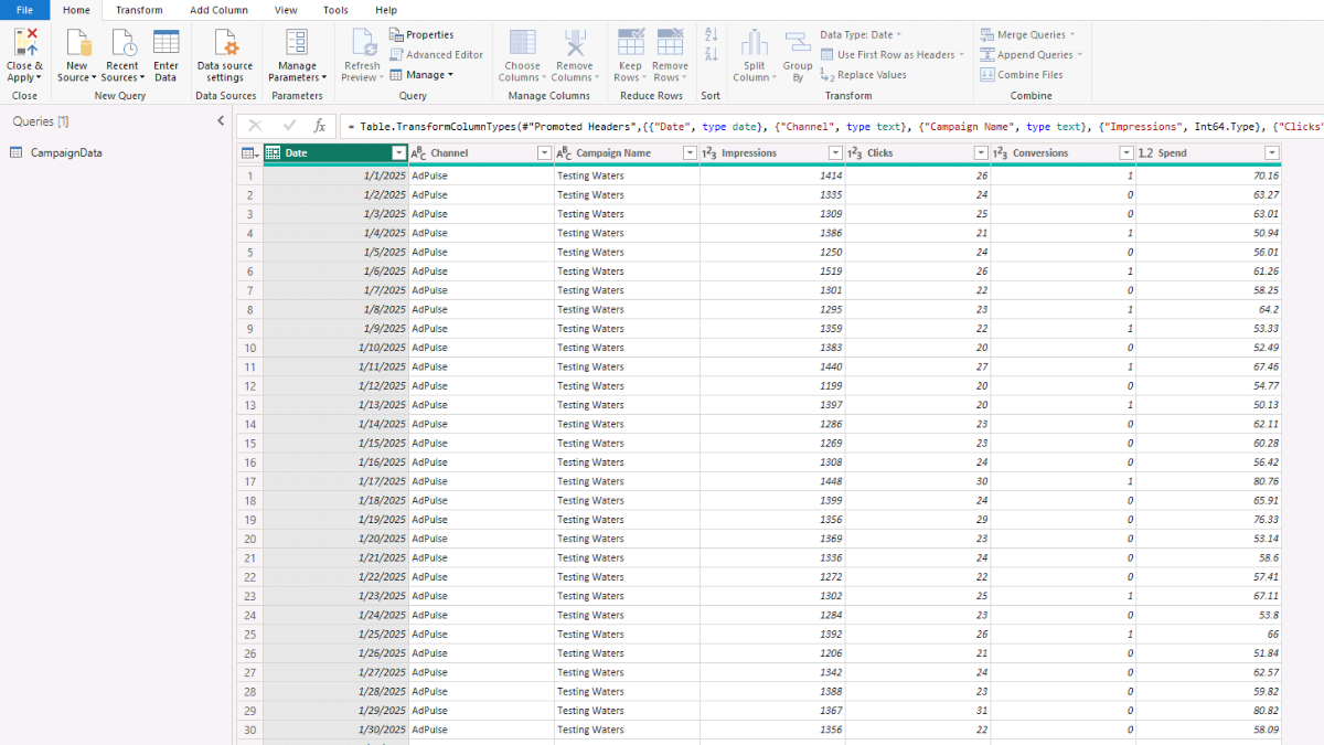
Next, go to the Home tab and select Close & Apply to load the data into Microsoft Power BI.

Note: This tutorial uses CSV files for simplicity, but you can also connect to other data sources such as SQL Server, SharePoint, or a data warehouse depending on your environment.

Step 2. Create DAX Tables and Build the Data Model

Now that the campaign data is loaded, we’ll create a few DAX tables and link them together into a clean Microsoft Power BI data model.

First, we’ll add a Calendar table, which wasn’t included in the original dataset. It will generate a continuous range of dates covering the actual data plus five additional years for budgeting and forecasting — which we’ll use later in the tutorial.

In Power BI’s Model view, select New Table from the Home tab and enter the following DAX code:

Calendar = 
VAR MinActualDate =
    CALCULATE ( MIN ( 'CampaignData'[Date] ), ALL ( 'CampaignData' ) )
VAR MaxActualDate =
    CALCULATE ( MAX ( 'CampaignData'[Date] ), ALL ( 'CampaignData' ) )
VAR StartDate = DATE ( YEAR ( MinActualDate ), 1, 1 )
VAR EndDate   = DATE ( YEAR ( MaxActualDate ) + 5, 12, 31 )
RETURN
ADDCOLUMNS (
    CALENDAR ( StartDate, EndDate ),
    "Year", YEAR ( [Date] ),
    "Month Name", FORMAT ( [Date], "MMMM" ),
    "Year-Month", FORMAT ( [Date], "yyyy-MM" ),
    "isActual",
        VAR d = [Date]
        RETURN IF ( d >= MinActualDate && d <= MaxActualDate, TRUE (), FALSE () ),
    "isForecast",
        VAR d = [Date]
        RETURN IF ( d > MaxActualDate && d <= EndDate, TRUE (), FALSE () )
)

Press Enter, and you’ll see a new table appear in the Model view and Data pane on the right. Right-click the table and select Mark as date table, then choose Date as the date field.

Next, let’s add two simple lookup tables to make filtering and analysis easier. Create a new table and paste the following DAX:

DimCampaign = 
DISTINCT (
    SELECTCOLUMNS (
        'CampaignData',
        "Campaign Name", 'CampaignData'[Campaign Name]
    )
)

Then repeat for marketing channels:

DimChannel = 
DISTINCT (
    SELECTCOLUMNS (
        'CampaignData',
        "Channel", 'CampaignData'[Channel]
    )
)

We now have four tables — one fact table (CampaignData) and three lookup (dimension) tables (Calendar, DimCampaign, and DimChannel). The fact table holds the raw performance metrics, while the dimension tables provide structured ways to filter and group the data.

In the Model view, drag Calendar[Date] onto CampaignData[Date]. Confirm that the relationship type is one-to-many, with single cross-filter direction, and mark it as active.

Repeat the process for DimCampaign[Campaign Name] → CampaignData[Campaign Name] and DimChannel[Channel] → CampaignData[Channel].

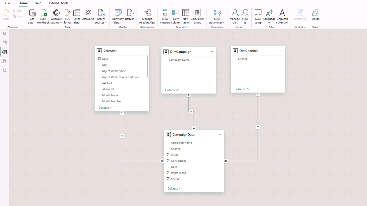
You now have a complete Microsoft Power BI data model ready to calculate performance indicators and analyze campaign data across multiple dimensions.

Step 3. Create Marketing Performance Indicators in DAX

We’re now ready to add measures that evaluate campaign performance. We’ll start with totals (impressions, clicks, conversions, and spend) and then calculate CTR, Conversion Rate, and CAC (Actual).

Create a small container table for measures in the Report view: go to Home → Enter data, name it Measures_Table, and click Load. In the Data pane, right-click Measures_Table and select New measure for each formula below.

Base aggregations
These four measures sum the core daily metrics from CampaignData. They respect any filters you apply (date, channel, or campaign), so they’re safe to use in all visuals that compare months or channels.

Impressions (Total) = 
SUM ( 'CampaignData'[Impressions] )

Clicks (Total) = 
SUM ( 'CampaignData'[Clicks] )

Conversions (Total) = 
SUM ( 'CampaignData'[Conversions] )

Spend (Total) = 
SUM ( 'CampaignData'[Spend] )

Performance indicators
These translate the base totals into marketing KPIs we’ll chart on the dashboard.

CTR — click-through rate: out of all impressions, what share produced a click.

CTR = 
VAR Clicks = [Clicks (Total)]
VAR Impressions = [Impressions (Total)]
RETURN
    DIVIDE ( Clicks, Impressions )

Conversion Rate — efficiency from click to conversion: out of all clicks, what share converted.

Conversion Rate = 
DIVIDE ( [Conversions (Total)], [Clicks (Total)] )

CAC (Actual) — historical customer acquisition cost: how much we paid (spend) for each conversion.

CAC (Actual) = 
DIVIDE ( [Spend (Total)], [Conversions (Total)] )

In the next step, we’ll build a report to explore these metrics by month and by channel.

Step 4. Build a Report to Analyze Campaign Performance

Start with a monthly matrix. In the Report view, add a Matrix visual. Put Calendar → Start of Month in Rows and add these measures to Values: Impressions (Total), Clicks (Total), Conversions (Total), Spend (Total), CTR, Conversion Rate, CAC (Actual). Format Start of Month as yyyy-MM (Format pane → Data format). If needed, right-click a column header and choose Rename for this visual to shorten labels.

Copy the matrix and switch Rows from Start of Month to DimChannel → Channel. This version compares performance by channel using the same KPIs (CTR, Conversion Rate, CAC).

Add a Slicer with DimChannel → Channel and set Style = Tile. This makes switching between channels quick and keeps interactions clear.

For a quick CAC breakdown by channel, insert a Treemap with Channel in Category and CAC (Actual) in Values.

To show spend trends and mix over time, add a Line and stacked column chart with Calendar → Year-Month on the X-axis, Spend (Total) on the Column Y-axis, and Channel as the Column legend. The columns show total spend per month, while colors indicate the channel mix.

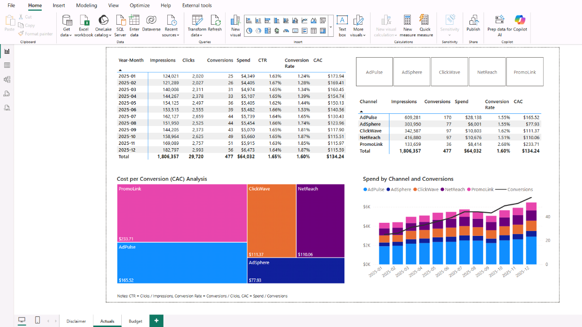
Insight to look for: if spend ramps to around $6 k toward year-end while Conversion Rate improves and Customer Acquisition Cost (CAC) declines, the incremental budget is working. If a channel such as AdPulse costs more but contributes over a third of conversions, consider keeping it for scale while removing underperformers (for example, Promolink). With that removal, CAC in the last three months settles near $110 — a reasonable starting point for the Budget and Forecast steps.

Step 5. Set Up Parameters for Customer Acquisition Projections

We’ll create a small set of drivers for the budget and forecast. These parameters will feed the DAX measures in the next step and let you run quick what-if checks.

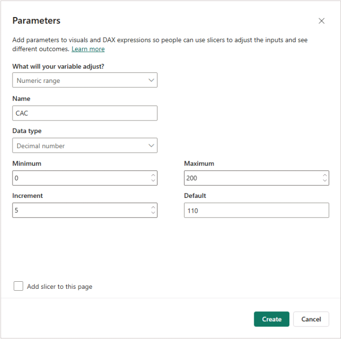
In Microsoft Power BI (Modeling tab), choose New parameter → Numeric range and create the first parameter:

• Name: CAC
• Data type: Decimal number
• Minimum: 0
• Maximum: 200
• Increment: 5
• Default: 110

Uncheck Add slicer to this page and click Create. A new CAC table will appear in the Data pane.

Now repeat the same process for the remaining parameters:

• Customer MRR — Min 0, Max 100, Increment 1, Default 6
• Monthly Budget — Min 0, Max 100 000, Increment 1 000, Default 9 000
• Monthly Churn — Min 0, Max 0.3, Increment 0.01, Default 0.03
• Users at Month 0 — Min 0, Max 10 000, Increment 100, Default 0

Note: Users at Month 0 represents the beginning-of-forecast active user base carried forward from your latest actuals.

Create a new report page (Budget). Add a Slicer and point it to Monthly Budget. In the Format pane, enable Single value and Slider. Repeat for CAC, Customer MRR, Monthly Churn, and Users at Month 0. This gives you a simple assumptions panel that will drive the forecast visuals.

Step 6. Forecasting Customer Growth and Revenue in Microsoft Power BI

We now need to set up several DAX measures to complete the marketing budget and forecast. In a nutshell, we’ll use the Power BI parameters to calculate the budget and forecast metrics.

For example, to estimate the number of new users in a given month, the model takes the monthly marketing budget (for example, $9,000) and divides it by the CAC (for example, $110). That gives a projection of approximately 82 new users added in that month.

We’ll assume a subscription-based service model. Each customer generates a monthly recurring fee (driven by the Customer MRR parameter) and is subject to a monthly churn rate (driven by the Monthly Churn parameter).

The goal is to project churned users and monthly revenue. The beginning-of-month (BOM) users represent the ending balance (EOM) from the previous month. From there, we add new users and adjust for churn to determine the number of active (EOM) customers.

The active (EOM) customers and the monthly MRR assumption together drive the monthly revenue forecast.

Note: The measures below use ISINSCOPE('Calendar'[Start of Month]) to ensure month-level rows and visual totals calculate correctly. Totals iterate months with SUMX rather than reusing a single month’s value. You can read more about this and other functions in DAX Guide [external link].

Step 6b. Building the Monthly Marketing Budget with DAX

Forecast Start (Month) — Defines the first forecast month immediately following the last actual date.

Forecast Start (Month) = 
VAR MaxActualDate =
    CALCULATE ( MAX ( 'CampaignData'[Date] ), ALL ( 'CampaignData' ) )
RETURN EOMONTH ( MaxActualDate, 0 ) + 1

Budget (Forecast) — Returns the monthly budget for each month.

Budget (Forecast) = 
VAR MonthlyBudget = 'Monthly Budget'[Monthly Budget Value]
RETURN
IF (
    ISINSCOPE ( 'Calendar'[Start of Month] ),
    MonthlyBudget,
    SUMX ( VALUES ( 'Calendar'[Start of Month] ), MonthlyBudget )
)

Users (BOM, Forecast) — Users at the beginning of each month.

Users (BOM, Forecast) = 
VAR fs  = [Forecast Start (Month)]
VAR mEval =
    IF (
        ISINSCOPE ( 'Calendar'[Start of Month] ),
        MAX ( 'Calendar'[Start of Month] ),                                   -- month row
        CALCULATE ( MIN ( 'Calendar'[Start of Month] ), STARTOFYEAR ( 'Calendar'[Date] ) )  -- BOY on totals
    )
RETURN
IF (
    ISBLANK ( mEval ) || mEval < fs,
    BLANK (),
    VAR r    = 'Monthly Churn'[Monthly Churn Value]
    VAR dec  = 1 - r
    VAR t    = DATEDIFF ( fs, mEval, MONTH )                   -- 0 for the first forecast month
    VAR U0   = 'Users at Month 0'[Users at Month 0 Value]
    VAR NU   = DIVIDE ( 'Monthly Budget'[Monthly Budget Value], 'CAC'[CAC Value] )
    VAR initial = U0 * POWER ( dec, t )
    VAR priorNew =
        IF (
            t > 0,
            SUMX (
                GENERATESERIES ( 0, t - 1 ),
                VAR i = [Value]
                VAR rem = ( t - 1 ) - i
                RETURN NU * POWER ( dec, rem )
            ),
            0
        )
    RETURN initial + priorNew
)

New Users (Monthly, Forecast) — Calculates new users each month based on Monthly Budget ÷ CAC, starting from the forecast start month.

New Users (Monthly, Forecast) = 
VAR fs = [Forecast Start (Month)]
RETURN
IF (
    ISINSCOPE ( 'Calendar'[Start of Month] ),
    IF ( MAX('Calendar'[Start of Month]) < fs, BLANK(),
         DIVIDE ( 'Monthly Budget'[Monthly Budget Value], 'CAC'[CAC Value] ) ),
    SUMX (
        VALUES ( 'Calendar'[Start of Month] ),
        VAR m = 'Calendar'[Start of Month]
        RETURN IF ( m < fs, BLANK(),
                    DIVIDE ( 'Monthly Budget'[Monthly Budget Value], 'CAC'[CAC Value] ) )
    )
)

Churn (Monthly, Forecast) — Churned users per month, calculated as BOM users × Monthly Churn rate.

Churn (Monthly, Forecast) = 
IF (
    ISINSCOPE ( 'Calendar'[Start of Month] ),
    VAR bom = [Users (BOM, Forecast)]
    RETURN IF ( ISBLANK ( bom ), BLANK(), bom * 'Monthly Churn'[Monthly Churn Value] ),
    SUMX (
        VALUES ( 'Calendar'[Start of Month] ),
        VAR bomM = CALCULATE ( [Users (BOM, Forecast)] )
        RETURN IF ( ISBLANK ( bomM ), BLANK(), bomM * 'Monthly Churn'[Monthly Churn Value] )
    )
)

Users (EOM, Forecast) — End-of-month users = BOM + New Users − Churn. (Totals return end-of-year values.)

Users (EOM, Forecast) = 
VAR mEOM =
    VAR bom  = [Users (BOM, Forecast)]
    VAR newU = [New Users (Monthly, Forecast)]
    VAR ch   = [Churn (Monthly, Forecast)]
    RETURN IF ( ISBLANK ( bom ) || ISBLANK ( newU ) || ISBLANK ( ch ), BLANK(), bom + newU - ch )
RETURN
IF (
    ISINSCOPE ( 'Calendar'[Start of Month] ),
    mEOM,
    CALCULATE ( mEOM, ENDOFYEAR ( 'Calendar'[Date] ) )
)

Revenue (Forecast, EOM) — Monthly forecasted revenue, calculated as EOM users × Customer MRR.

Revenue (Forecast, EOM) = 
IF (
    ISINSCOPE ( 'Calendar'[Start of Month] ),
    [Users (EOM, Forecast)] * 'Customer MRR'[Customer MRR Value],
    SUMX (
        VALUES ( 'Calendar'[Start of Month] ),
        CALCULATE ( [Users (EOM, Forecast)] ) * 'Customer MRR'[Customer MRR Value]
    )
)

Let’s now put these DAX measures into practice in the marketing budget dashboard.

Tip: To stay organized, create subfolders for your Actual and Forecast measures. In Power BI’s Model view, select a measure and enter Actuals or Forecast in the Display Folder field under Properties. The folders will appear in the Data pane, and you can drag other measures into them for easy management.

Step 7. Completing the Budget Dashboard with Key Customer Metrics

We’ll assemble the monthly Budget table and add a compact Customer Metrics summary so you can see how assumptions affect LTV and ROI.

1. Create a Matrix in the Report view. Add Calendar → Start of Month to Rows (format as yyyy-MM). Add these measures to Values:
   Budget (Forecast), Users (BOM, Forecast), New Users (Monthly, Forecast), Churn (Monthly, Forecast), Users (EOM, Forecast), Revenue (Forecast, EOM).
   Use Rename for this visual if you want shorter labels.
2. Add a Slicer with Calendar → Year and set the slicer style to Dropdown. Adjust parameters (for example, CAC and Monthly Budget) to see the projections update.

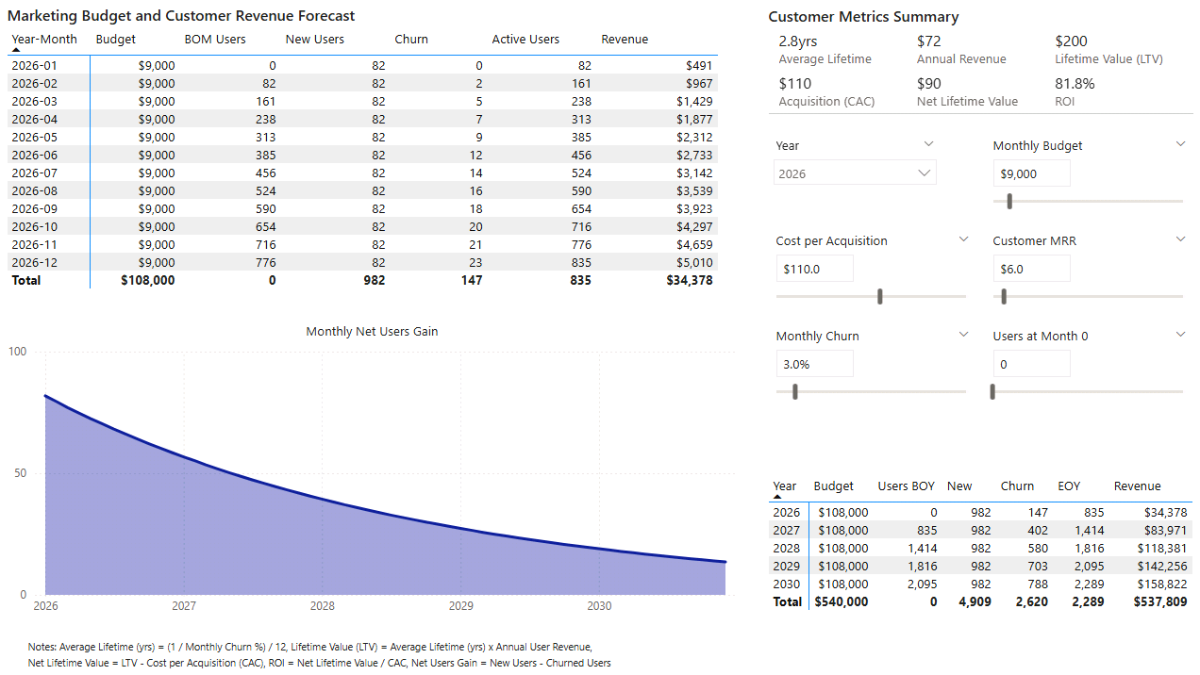
Now add a Multi-row card for a compact Customer Metrics summary. Use the measures below (DAX unchanged) with a short description of what each shows.

Average Lifetime (Months, Forecast) — expected customer lifetime in months at the current churn rate.

Average Lifetime (Months, Forecast) = 
DIVIDE ( 1, 'Monthly Churn'[Monthly Churn Value] )

Average Lifetime (Years, Forecast) — the same metric expressed in years.

Average Lifetime (Years, Forecast) = 
DIVIDE ( [Average Lifetime (Months, Forecast)], 12 )

Customer Annual Revenue (Forecast) — ARPU per year from the current monthly revenue assumption.

Customer Annual Revenue (Forecast) = 
'Customer MRR'[Customer MRR Value] * 12

LTV (Undiscounted, Forecast) — simple lifetime value: monthly revenue × expected lifetime (months).

LTV (Undiscounted, Forecast) = 
'Customer MRR'[Customer MRR Value] * [Average Lifetime (Months, Forecast)]

Net LTV (Undiscounted, Forecast) — contribution per customer before other costs: LTV − CAC.

Net LTV (Undiscounted, Forecast) = 
VAR ltv = [LTV (Undiscounted, Forecast)]
VAR cac = 'CAC'[CAC Value]
RETURN IF ( ISBLANK ( ltv ) || ISBLANK ( cac ), BLANK (), ltv - cac )

ROI (Forecast) — simple ROI relative to the Customer Acquisition Cost (CAC).

ROI (Forecast) = 
DIVIDE ( [LTV (Undiscounted, Forecast)], 'CAC'[CAC Value] ) - 1

This completes the budget view: a monthly table you can filter by year, plus a metrics card that explains the economics behind your assumptions. Next, we’ll aggregate to annual totals and add a quick sensitivity check.

Step 8. Long-term Marketing Spend Forecast and Sensitivity Analysis

We’ll convert the monthly forecast into annual totals and add a quick net-gain view. Then we’ll close with a short sensitivity example to show how CAC and churn impact ROI.

Annual forecast (table)
Insert a Matrix visual and display results by year. Add the measures below (DAX unchanged) — brief descriptions explain what each returns.

Users (BOY, Forecast, by Year) — beginning-of-year users based on the monthly BOM logic.

Users (BOY, Forecast, by Year) = 
CALCULATE (
    [Users (BOM, Forecast)],
    STARTOFYEAR ( 'Calendar'[Date] )
)

New Users (Annual, Forecast) — total new users across months in the year.

New Users (Annual, Forecast) = 
SUMX (
    VALUES ( 'Calendar'[Start of Month] ),
    [New Users (Monthly, Forecast)]
)

Churn (Annual, Forecast) — total churned users across months in the year.

Churn (Annual, Forecast) = 
SUMX (
    VALUES ( 'Calendar'[Start of Month] ),
    [Churn (Monthly, Forecast)]
)

Users (EOY, Forecast, by Year) — end-of-year users = BOY + New − Churn.

Users (EOY, Forecast, by Year) = 
[Users (BOY, Forecast, by Year)] + [New Users (Annual, Forecast)] - [Churn (Annual, Forecast)]

Revenue (Annual, Forecast, EOM) — annual revenue (sum of monthly forecast revenue).

Revenue (Annual, Forecast, EOM) = 
SUMX (
    VALUES ( 'Calendar'[Start of Month] ),
    [Revenue (Forecast, EOM)]
)

Net user gain (chart)
Add an Area chart with Calendar → Start of Month on the X-axis and the measure below on the Y-axis to visualize acquired minus churned users over time.

Net User Gain (Forecast) = 
[New Users (Monthly, Forecast)] - [Churn (Monthly, Forecast)]

Tip: To disconnect the Year slicer from the annual tables or the area charts, select the slicer → Format → Edit interactions and set None (one of the two icons in the upper-right corner) on those visuals.

Sensitivity snapshot
Assume a Monthly Budget of $9,000. With Monthly Churn = 3.0% and Customer MRR = $6.00, the undiscounted LTV is about $200, giving an ROI ≈ 82% when CAC = $110. If CAC rises to $135 (~+20%), ROI drops to ~48.1%. Increasing Monthly Churn from 3% → 4% can bring ROI down further to ~11.1%.

Since this simple ROI excludes other operating costs beyond CAC, such declines are a concern and worth testing with different parameter settings.

📌 Recap: Building a Marketing Performance and Forecast Model in Microsoft Power BI

Here’s a quick recap of the steps we followed to build a complete online campaign performance and customer acquisition forecast model in Microsoft Power BI:

1. Import Campaign Data. Load your marketing performance CSV file into Power BI and review metrics like impressions, clicks, conversions, and spend.
2. Create DAX Tables and Relationships. Build Calendar, Channel, and Campaign dimension tables, and link them to the campaign data for a clean star schema model.
3. Build Core DAX Measures. Define total impressions, clicks, conversions, spend, CTR, Conversion Rate, and CAC (Actual) to evaluate campaign performance.
4. Design the Campaign Dashboard. Use matrices and visuals to analyze monthly performance and compare key marketing channels side by side.
5. Set Up Forecast Parameters. Create Power BI parameters for CAC, Monthly Budget, Customer MRR, Churn, and Users at Month 0 to drive interactive assumptions.
6. Create Forecast Measures. Use DAX to model monthly customer acquisition, churn, and projected revenues based on the budget and parameters.
7. Complete the Budget Dashboard. Combine forecast tables and KPI cards to show customer lifetime value (LTV), ROI, and revenue forecasts.
8. Build Annual Projections and Sensitivity Analysis. Aggregate monthly data into yearly forecasts and test how changes in CAC or churn affect profitability.

By following these steps, you’ve built a Power BI model that tracks marketing performance, projects customer growth, and visualizes long-term ROI under different budget and churn scenarios.

📥 Download My Marketing Performance & Forecast Data Template

To help you get started faster, I’ve prepared a ready-to-use Power BI package that includes everything you need:

• Power BI (.pbix) file with the full marketing performance and forecasting model, including parameters, DAX measures, and dashboards.
• CSV data source for campaign metrics so you can instantly load and explore the model.
• Text file with all DAX measures neatly organized for easy reference and reuse.

This package lets you analyze marketing performance, forecast customer growth, and test different acquisition and budget scenarios directly in Microsoft Power BI.

👁️ View full template details

Get in Touch

Hi, I’m Jacek. I’m passionate about Microsoft Power BI, DAX, and data-driven marketing analytics! I hope this tutorial helped you understand how to connect campaign data, build interactive dashboards, and forecast customer acquisition with dynamic assumptions.

Feel free to get in touch if you have any questions about Power BI, forecasting, or marketing analytics.

You can also explore my other tutorials for more step-by-step guides, or check out my One-to-One Training and Data Analytics Support if you’d like personalized help.

Disclaimer: This tutorial is for informational and educational purposes only and should not be considered professional advice.

Explore More Tutorials

• Power BI Customer Churn & Revenue Forecast Tutorial — Build a Power BI model to analyze churn, retention, and forecast recurring revenue using DAX measures and parameters.
• Excel Monthly Budget & Forecast Tutorial — Create a dynamic budget and forecast model in Excel to track spend and analyze trends month by month.
• Excel Marketing Investment Plan Tutorial — Design an Excel model to plan and monitor marketing budgets and ROI across channels.
• Subscription Model with Churn Calculation — Learn how to model subscriptions and retention dynamics in Excel.
• Excel Churn & Retention Cohort Analysis Tutorial — Perform retention and churn cohort analysis to understand customer behavior over time.