Last Updated on February 21, 2026
In this tutorial, we will build a complete Financial Planning and Analysis (FP&A) dashboard in Microsoft Power BI using a realistic dataset that includes daily profit and loss activity, monthly cash flow and balance sheet data, and a detailed payroll roster. This will give us a practical foundation to create dynamic financial reporting and forecasting across the full P&L, cash flow, and balance sheet.
We’ll begin by loading and shaping the data, building a clean star-schema model, and creating DAX dimensions that mirror how FP&A teams structure financial models. From there, we will calculate actual financial performance, introduce key planning parameters, and build a set of forecasting measures for revenue, operating expenses, payroll, capital expenditure, depreciation, working capital, and debt.
By the end, you’ll have a multi-page Microsoft Power BI dashboard that tracks actual results, visualizes operational drivers, and projects future performance through a full P&L, cash flow, and balance sheet forecast.
🔎 You can preview the dashboard to follow along or watch my FP&A Dashboard Video Tutorial at the end of this tutorial.
Table of Contents
Step 1. Loading and Exploring the FP&A Data in Microsoft Power BI
We begin our build by loading the core FP&A dataset into Microsoft Power BI Desktop. The demo files represent a fast-growing company operating throughout 2025, with daily profit and loss activity, monthly cash flow and balance sheet data, and a detailed payroll roster.
Together, these sources provide a realistic foundation for financial planning, financial analysis, and cash flow forecasting.
Step 1a. Importing Financial Data into Microsoft Power BI
Open Microsoft Power BI Desktop and load each of the prepared files (Home → Get Data → Text/CSV), so you can examine their structure before modeling.
For this Financial Planning and Analysis Dashboard, I used the following four source files:
- pnl_daily_2025 – Daily P&L entries for 2025, including subscription revenue, license sales, services income, cost of goods sold, payroll, operating expenses, and depreciation.
- cash_flow_monthly_2025 – Monthly cash flow statement (indirect method), containing Net Income, D&A, Working Capital movements, CapEx, and equity funding.
- balance_sheet_monthly_2025 – Monthly balance sheet with cash, accounts receivable, deferred revenue, accounts payable, PPE, equity, and retained earnings.
- payroll_roster_2025 – Employee-level payroll roster including hire dates, department, salary, bonus %, and employer costs.
After reviewing the dataset previews, click Load to bring the data into the model.
📥 You can download the source files and the completed Power BI dashboard file at the end of this tutorial.
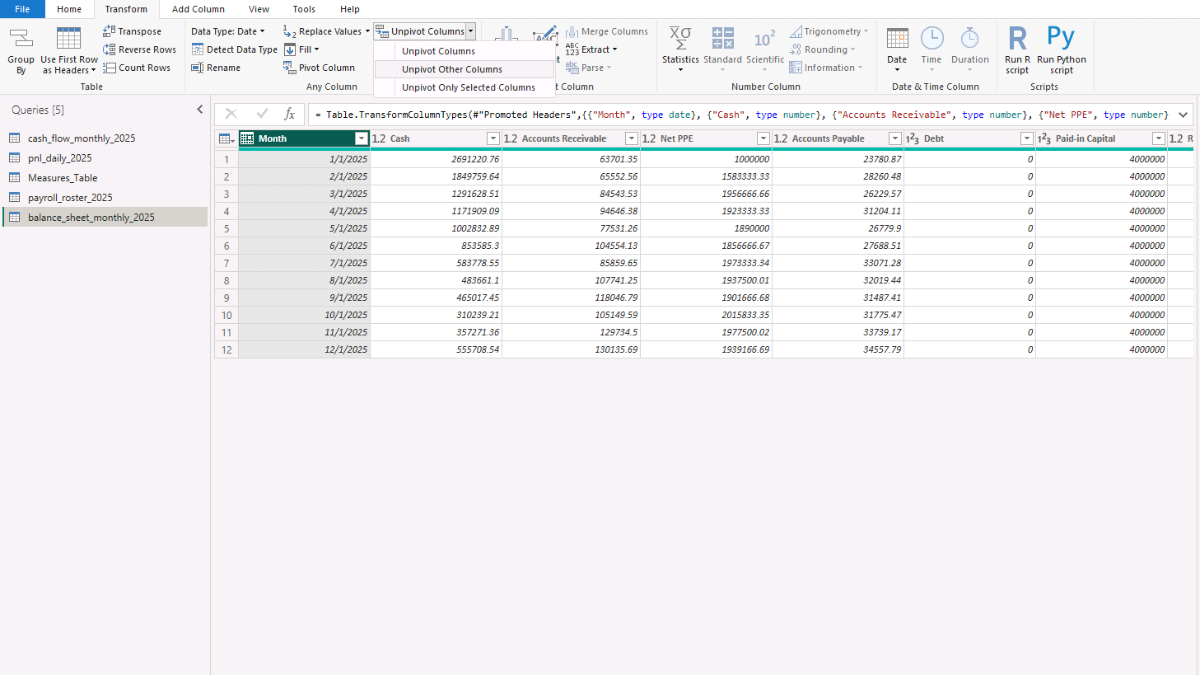
Step 1b. Reshaping Balance Sheet Data in Power Query
The balance sheet file arrives in a “wide” format where each balance sheet line appears as a separate column. For financial reporting and dashboarding, it is more flexible to convert this into a “long” structure with three fields: Month | Category | Amount.
This structure works much better for a matrix visual, enables slicers by balance-sheet line item, and simplifies later DAX calculations.
To reshape the data:
- From Home → Get Data → Text/CSV, select balance_sheet_monthly_2025.csv and choose Transform Data.
- In Power Query, select the Month column.
- Go to Transform → Unpivot Columns → Unpivot Other Columns.
- Rename the auto-generated fields: Attribute → Category, Value → Amount
- Set correct data types (Month = Date, Category = Text, Amount = Decimal Number).
- Click Close & Apply.
If you want to reproduce the transformation programmatically, here is the optional M code:
let
    Source = Csv.Document(File.Contents("balance_sheet_monthly_2025.csv"),[Delimiter=",", Columns=??, Encoding=65001, QuoteStyle=QuoteStyle.Csv]),
    PromotedHeaders = Table.PromoteHeaders(Source, [PromoteAllScalars=true]),
    ChangedTypes = Table.TransformColumnTypes(PromotedHeaders,{{"Month", type date}}),
    Unpivoted = Table.UnpivotOtherColumns(ChangedTypes, {"Month"}, "Category", "Amount"),
    FinalTypes = Table.TransformColumnTypes(Unpivoted, {{"Category", type text}, {"Amount", type number}})
in
    FinalTypes
Note: Before continuing, go to: File → Options and Settings → Options → Current File → Data Load and uncheck “Autodetect new relationships after data is loaded.” We will build all relationships manually so you can fully understand how the financial planning model operates inside Power BI.
Step 2. Creating a Dynamic Calendar Table for Financial Modeling
A robust financial dashboard requires a proper calendar table. In FP&A work, every measure—whether from the P&L, cash flow, balance sheet, or forecast—needs to align on a consistent time dimension. Microsoft Power BI handles time-intelligence functions best when you provide a dedicated date table rather than relying on dates embedded in fact tables.
In this step, we will create a dynamic calendar using DAX. The table automatically detects the earliest and latest dates from the P&L actuals and then extends the range five years into the future. This ensures our model supports both actual analysis and long-range financial planning.
To create the table, go to the Power BI’s Model view → New Table and enter the following DAX:
Calendar =
VAR _MinDate =
    MINX ( ALL ( pnl_daily_2025 ), pnl_daily_2025[Date] )
VAR _MaxActualDate =
    MAXX ( ALL ( pnl_daily_2025 ), pnl_daily_2025[Date] )
RETURN
ADDCOLUMNS (
    CALENDAR ( _MinDate, DATE ( YEAR ( _MaxActualDate ) + 5, 12, 31 ) ),
    "Year",         YEAR ( [Date] ),
    "MonthNo",      MONTH ( [Date] ),
    "Month",        FORMAT ( [Date], "MMMM" ),
    "Quarter",      "Q" & FORMAT ( [Date], "Q" ),
    "YearMonth",    FORMAT ( [Date], "YYYY-MM" ),
    "YearMonthNum", YEAR ( [Date] ) * 100 + MONTH ( [Date] ),
    "MonthStart",   DATE ( YEAR ( [Date] ), MONTH ( [Date] ), 1 ),
    "MonthEnd",     EOMONTH ( [Date], 0 ),
    "IsActual",     [Date] <= _MaxActualDate,
    "IsForecast",   [Date] > _MaxActualDate
)
This expression uses the CALENDAR function to generate a continuous date range and ADDCOLUMNS to enrich the table with attributes essential for financial analysis—such as MonthStart and MonthEnd, numerical YearMonth keys, and flags distinguishing actual months from forecast months.
After creating the table, right-click Calendar → Mark as date table and select the Date column. This ensures Microsoft Power BI recognises it as your primary time dimension and activates full time-intelligence functionality.
Step 3. Building the Financial Data Model for FP&A Reporting
With our datasets loaded and the calendar table in place, we can now begin assembling the financial data model. In FP&A reporting, a clean, well-structured model is crucial because it allows us to aggregate actuals, analyse operational drivers, and layer on forecasting logic without ambiguity.
Following a star-schema approach, we will organise the model around central fact tables connected to supporting dimensions, with the Calendar table acting as the primary time dimension. The aim is to keep the fact tables additive and streamlined, while the DAX dimensions provide structure for slicing, grouping, and visualising financial performance across the profit and loss, cash flow, and balance sheet.
Step 3a. Understanding the Fact and Dimension Structure
Core Dimension
- Calendar — Controls all time intelligence and defines the forecast horizon.
Fact Tables
- pnl_daily_2025 — Daily Profit & Loss transactions.
- cash_flow_monthly_2025 — Monthly cash flow (indirect method).
- balance_sheet_monthly_2025 — Month-end balance sheet values.
- payroll_roster_2025 — Employee-level payroll and headcount details.
Step 3b. Creating Relationships for Financial Reporting
We now join the tables using the Calendar table as the central dimension:
Model Relationships (Cardinality: 1:*, Direction: Single):
- Calendar[Date] → pnl_daily_2025[Date]
- Calendar[Date] → cash_flow_monthly_2025[Month]
- Calendar[Date] → balance_sheet_monthly_2025[Month]
- Calendar[Date] → payroll_roster_2025[HireDate]
These relationships allow us to analyse daily P&L activity, monthly cash flow, and month-end balance sheet positions consistently across the same time dimension.
Payroll is linked through hire dates, enabling us to calculate month-end headcount and project future staffing levels.
Your model should now resemble a clean financial star schema where the Calendar table drives all time-based logic, fact tables remain fully additive and unambiguous for straightforward DAX development, and financial analysis stays consistent across the P&L, cash flow, and balance sheet.
Step 4. Creating Financial Dimensions Using DAX
With the foundational data model in place, the next step is to add a set of custom DAX dimension tables. They will make it possible to build clear reporting hierarchies, apply custom sorting, and create consistent financial groupings that do not exist natively in the raw fact tables.
In Microsoft Power BI, we can create these tables directly in the model using DAX. This approach gives us full control over how financial categories are defined, ordered, and related to one another.
To begin, go to Model view → New table and enter the DAX expressions below.
Step 4a. Creating Balance Sheet Dimension Tables
This table provides a controlled list of balance sheet line items, grouped into Assets, Liabilities, and Equity.
It also includes a DisplayOrder field so the balance sheet appears in the correct accounting order in visuals.
DimBS_Category =
DATATABLE (
    "Category", STRING, "Section", STRING, "DisplayOrder", INTEGER,
    {
        { "Cash",                "Assets",      10 },
        { "Accounts Receivable", "Assets",      20 },
        { "Net PPE",             "Assets",      30 },
        { "Accounts Payable",    "Liabilities", 60 },
        { "Debt",                "Liabilities", 70 },
        { "Paid-in Capital",     "Equity",      90 },
        { "Retained Earnings",   "Equity",     100 }
    }
)
Sorting: Select Category → Sort by column → DisplayOrder.
Relationship: DimBS_Category[Category] → balance_sheet_monthly_2025[Category]. Cardinality: 1:*, Direction: Single.
Step 4b. Creating Profit & Loss Dimension Tables
To support a structured and properly ordered Profit & Loss statement, we create two small dimension tables. DimPL_Subcategory organizes detailed P&L subcategories with their associated account codes, while DimPL_Account groups those subcategories into higher-level accounts and assigns a display order for reporting.
DimPL_Subcategory: This dimension extracts unique P&L subcategories from the daily ledger and includes the account and account code fields, allowing you to enforce a consistent financial statement order.
DimPL_Subcategory =
DISTINCT (
    SELECTCOLUMNS (
        pnl_daily_2025,
        "Subcategory",  pnl_daily_2025[Subcategory],
        "Account",      pnl_daily_2025[Account],
        "AccountCode",  pnl_daily_2025[AccountCode]
    )
)
Sorting: Sort Subcategory by AccountCode.
Relationship: DimPL_Subcategory[Subcategory] → pnl_daily_2025[Subcategory]
DimPL_Account: This table creates a list of high-level P&L accounts (Revenue, COGS, Opex, etc.) and calculates a DisplayOrder based on the first digits of the account code. This ensures categories appear in financial statement order.
DimPL_Account =
ADDCOLUMNS (
    SUMMARIZE ( pnl_daily_2025, pnl_daily_2025[Account] ),
    "DisplayOrder",
        VAR MinCode = CALCULATE ( MIN ( pnl_daily_2025[AccountCode] ) )
        RETURN INT ( DIVIDE ( MinCode, 100, 0 ) )
)
Sorting: Sort Account by DisplayOrder.
Relationship: DimPL_Account[Account] → DimPL_Subcategory[Account]. Cardinality: 1:*, Direction: Single.
Step 4c. Creating a Cash Flow Dimension Table
This dimension creates a stable list of cash flow categories—Operating, Investing, Financing, and Net—along with the correct display order for reporting.
DimCF_Category =
ADDCOLUMNS (
    DISTINCT ( SELECTCOLUMNS ( cash_flow_monthly_2025, "Category", cash_flow_monthly_2025[Category] ) ),
    "DisplayOrder",
        SWITCH (
            TRUE(),
            [Category] = "Operating",  10,
            [Category] = "Investing",  20,
            [Category] = "Financing",  30,
            [Category] = "Net",        40,
            90
        )
)
Sorting: Sort Category by DisplayOrder.
Relationship: DimCF_Category[Category] → cash_flow_monthly_2025[Category]. Cardinality: 1:*, Direction: Single.
Step 4d. Creating the Department Dimension
This dimension extracts the list of departments from the payroll roster. It enables analysis of headcount, payroll cost, and productivity by functional area.
DimDepartment =
DISTINCT (
    SELECTCOLUMNS (
        payroll_roster_2025,
        "Department", payroll_roster_2025[Department]
    )
)
Relationship: DimDepartment[Department] → payroll_roster_2025[Department]. Cardinality: 1:*, Direction: Single.
Step 4e. Completed Power BI Data Model
Once you’ve loaded the Profit and Loss, Cash Flow, Balance Sheet, and Payroll datasets, created the Calendar table, and added the DAX dimensions, your final data model should look like the diagram below.
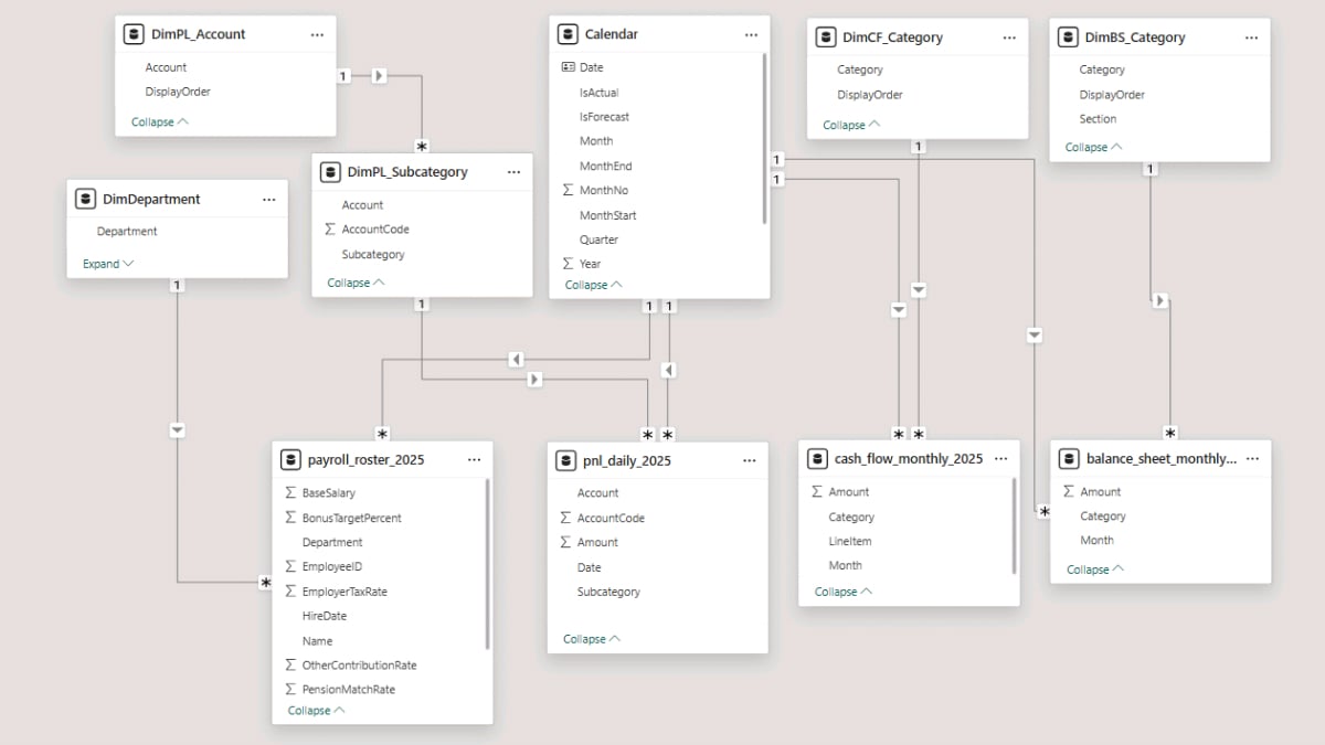
We can now begin developing the key financial measures that will drive both our actuals reporting and later forecasting.
Step 5. Developing Core Financial Measures with DAX
In FP&A work, measures form the analytical engine of the model: they calculate revenue, gross profit, operating expenses, cash flow, balance sheet values, and operational metrics such as headcount or productivity.
To keep the model organised, we will store all measures inside a dedicated table. In Report view, go to Home → Enter Data, name the table Measures_Table, and click Load.
Then, right-click the table and choose New measure to begin adding the expressions below.
Step 5a. Building Profit & Loss Actual Measures
This first group of measures calculates the core P&L values directly from the daily ledger. These serve as the foundation for all later performance metrics and forecasting logic. Common DAX patterns such as SUM, CALCULATE, ALL, KEEPFILTERS, and date filtering help ensure accurate aggregation of financial data.
-- Core Counts
PL Amount =
SUM ( pnl_daily_2025[Amount] )

Revenue =
CALCULATE(
    [PL Amount],
    ALL(DimPL_Account),
    DimPL_Account[Account] = "Revenue"
)

COGS =
CALCULATE(
    [PL Amount],
    ALL(DimPL_Account),
    DimPL_Account[Account] = "COGS"
)

Opex =
CALCULATE(
    [PL Amount],
    ALL(DimPL_Account),
    DimPL_Account[Account] = "Opex"
)

Payroll Cost =
CALCULATE (
    [PL Amount],
    KEEPFILTERS (
        DimPL_Subcategory[Subcategory] = "Payroll (incl. taxes/benefits/bonus accrual)"
        )
    )

Opex ex Payroll =
[Opex] - [Payroll Cost]

D&A =
CALCULATE(
    [PL Amount],
    ALL(DimPL_Account),
    DimPL_Account[Account] = "D&A"
)

Income Tax Expense =
CALCULATE(
    [PL Amount],
    ALL(DimPL_Account),
    DimPL_Account[Account] = "Tax"
)

Interest Expense =
CALCULATE(
    [PL Amount],
    ALL(DimPL_Account),
    DimPL_Account[Account] = "Interest"
)

Headcount (EOP) =
VAR _eop = MAX('Calendar'[Date])
RETURN
CALCULATE(
    DISTINCTCOUNT(payroll_roster_2025[EmployeeID]),
    REMOVEFILTERS('Calendar'),
    payroll_roster_2025[HireDate] <= _eop, OR( ISBLANK(payroll_roster_2025[TerminationDate]), payroll_roster_2025[TerminationDate] > _eop
        )
    )
--
With these base measures in place, we can now derive familiar FP&A indicators such as gross profit, EBITDA, net income, and per-employee productivity metrics.
-- Profit and loss performance metrics
Gross Profit =
[Revenue] + [COGS]

EBITDA  =
[Gross Profit] + [Opex]

EBIT  =
[EBITDA] + [D&A]

Net Income =
[EBIT] + [Income Tax Expense] + [Interest Expense]

Cost per Employee =
DIVIDE ( [Payroll Cost], [Headcount (EOP)] )

Revenue per Employee =
DIVIDE ( [Revenue], [Headcount (EOP)] )
--
Step 5b. Building Cash Flow Actual Measures
The next set of measures summarises the actual cash flow activity in the dataset. These represent the standard classifications used throughout financial analysis—Operating, Investing, and Financing—and will form the basis for the cash flow forecast later in the tutorial.
-- Cash Flow actual measures
CF Amount =
SUM ( cash_flow_monthly_2025[Amount] )

CFO =
CALCULATE(
    [CF Amount],
    ALL(DimCF_Category),
    DimCF_Category[Category] = "Operating"
)

CFI =
CALCULATE(
    [CF Amount],
    ALL(DimCF_Category),
    DimCF_Category[Category] = "Investing"
)

CFF =
CALCULATE(
    [CF Amount],
    ALL(DimCF_Category),
    DimCF_Category[Category] = "Financing"
)

Capex  =
CALCULATE(
    [CF Amount],
    ALL(DimCF_Category),
    DimCF_Category[Category] = "Investing"
)
--
Step 5c. Creating Balance Sheet Actual Measures
Now that we have cash flow results, we can move on to the balance sheet. The following measures calculate month-end balances for key line items such as assets, liabilities, and equity. These will also serve as the actuals baseline for the balance sheet forecast in later sections.
-- Balance Sheet actual measures
BS Amount (Monthly) =
SUM ( balance_sheet_monthly_2025[Amount] )

BS Amount =
VAR _month = MAX('Calendar'[MonthStart])
RETURN
    CALCULATE(
        [BS Amount (Monthly)],
        ALL('Calendar'),
        'Calendar'[MonthStart] = _month
    )

BS Total Assets =
CALCULATE(
    [BS Amount],
    DimBS_Category[Section] = "Assets",
    ALL(DimBS_Category[Category])
)

BS Total Liabilities =
CALCULATE(
    [BS Amount],
    DimBS_Category[Section] = "Liabilities",
    ALL(DimBS_Category[Category])
)

BS Total Equity =
CALCULATE(
    [BS Amount],
    DimBS_Category[Section] = "Equity",
    ALL(DimBS_Category[Category])
)

BS Balance Check =
[BS Total Assets] - [BS Total Liabilities] - [BS Total Equity]
--
Note: After creating your first measure, you can keep your model organised by placing measures into display folders. In Model view, click any measure, open the Properties pane, and type a folder name (e.g., Actual – Totals) into the Display folder field. Press Enter, and the measure will appear under a dedicated sub-folder. You can create additional folders for P&L, Cash Flow, Balance Sheet, or Forecast measures depending on your preferred structure.
Step 6. Actuals Analysis and Financial Reporting
With our actuals measures complete, we can now begin shaping the first part of the reporting dashboard. This section focuses entirely on historical results: a clearly formatted Profit and Loss statement, a Cash Flow statement, a Balance Sheet, and a set of analytical views exploring monthly performance and cost trends.
The goal is to replicate the structure and readability of a classic FP&A reporting pack — only now fully interactive within Microsoft Power BI.
Step 6a. Building the Financial Statements Power BI Dashboard
We will start by creating a dedicated page that groups all three primary financial statements together. Before adding any visuals, open the Filter pane and drag Calendar[IsActual] into the Filters on this page area, setting the filter to True. This ensures the entire page reports only historical data.
Profit and Loss Statement
The Profit and Loss matrix gives you a clean, month-by-month view of the company’s financial performance. By organising the rows with the DimPL_Account hierarchy and the columns with MonthStart, the visual becomes a compact but comprehensive summary of revenue, cost of goods sold, operating expenses, payroll, depreciation, and ultimately net income.
To build a Power BI Profit and Loss Statement, insert a Matrix visual and place DimPL_Account[Account] in the rows, followed by Calendar[MonthStart] in the columns. Then, add your PL Amount measure to the values.
Switching MonthStart to a yyyy-mm format in the Format pane improves readability and makes monthly trends easier to compare. You can refine the layout further by adjusting column header styles or enabling row subtotals—renaming the subtotal to Net Income, for example, creates a clear and intuitive finish to the statement.
If you want to tidy up labels, right-click any field name and use Rename for this visual.
Cash Flow Statement
The cash flow matrix summarises the company’s operating, investing, and financing movements using the indirect method. It helps you quickly compare P&L profitability with actual cash generation and understand how investing and financing decisions shape the month-end cash position.
To build a Power BI Cash Flow Statement, insert another Matrix — either start fresh or duplicate the P&L matrix to keep formatting consistent.
Place DimCF_Category[Category] in the rows and add the CF Amount measure to the values.
Make sure the title and labels reflect the structure of a Cash Flow Statement; you can adjust these at any time using Rename for this visual.

Balance Sheet Statement
The balance sheet visual highlights the company’s month-end financial position using both the high-level Section (Assets, Liabilities, Equity) and Category (Cash, Accounts Receivable, Net PPE, etc.) fields from your custom DAX dimension. This creates a structured and easily expandable overview of the organisation’s financial standing.
To build a Power BI Balance Sheet Statement, insert a Matrix, add Calendar[MonthStart] (formatted as yyyy-mm) to the columns, then place DimBS_Category[Section] in the rows followed by DimBS_Category[Category] beneath it. Add the BS Amount measure to the values, and adjust the matrix title and row labels as needed.
Step 6b. Financial Analysis and Insights
Next, let’s create a second page dedicated to analytical insights and name it Analysis. Apply the same page-level filter for Calendar[IsActual] = True to keep all visuals focused on historical results.
This visual provides a compact trend view of the P&L, letting you compare revenue, gross profit, operating expenses, D&A, and net income month over month. It complements the full P&L matrix by presenting performance in a condensed, analytical layout.
To build a monthly profit and loss view, insert a Matrix, place Calendar[MonthStart] in the rows, and add the core P&L measures—Revenue, COGS, Gross Profit, Opex, D&A, and Net Income—to the values. Format MonthStart as yyyy-mm and enable the title for clarity. The result is a clean month-by-month financial trend summary.
Annual Opex Analysis by Category
Operating expenses vary across categories, and this visual makes it easy to see which areas drive total spend. It’s an effective diagnostic view for assessing cost efficiency or identifying budget variances.
To build the opex analysis, insert a Clustered bar chart, place DimPL_Subcategory[Subcategory] on the Y-axis, and add PL Amount to the X-axis. Sorting the bars by PL Amount in ascending order quickly highlights the largest and smallest Opex contributors. Turning on data labels and choosing an appropriate display unit will further improve readability.

Monthly Headcount Breakdown by Department
This visual shows how staffing levels change across departments over time. It’s especially useful when total headcount looks stable overall but individual departments experience meaningful shifts throughout the year.
To build the headcount analysis, insert a Stacked column chart, add Calendar[MonthStart] to the X-axis and Headcount (EOP) to the Y-axis, then place DimDepartment[Department] in the Legend. Enable the legend in the Format pane and position it wherever it best fits your layout.
Monthly Payroll Cost Analysis
This visual brings together payroll cost, headcount, and per-employee productivity metrics to give you a clear view of workforce efficiency. It’s a common FP&A tool for tracking how payroll investment aligns with revenue generation.
To analyze payroll cost in Microsoft Power BI, insert a Matrix, add Calendar[MonthStart] to the rows, and include Revenue, Payroll Cost, Headcount (EOP), Revenue per Employee, and Cost per Employee in the values. Use Rename for this visual to tidy up labels, and adjust the column headers in the Format pane for a clean final presentation.
Step 7. Financial Planning and Forecasting in Microsoft Power BI
With the actuals reporting and analysis pages in place, we can now move into the second major phase of this tutorial: creating a fully integrated financial planning and analysis (FP&A) forecasting model inside Microsoft Power BI.
This section introduces the forecasting logic that will support revenue projections, cost planning, payroll modeling, headcount planning, depreciation schedules, debt calculations, and working capital forecasting. Together, these elements drive a complete forward-looking cash flow and balance sheet.
Before we can build the forecast visuals in the next step, we first need to set up the parameters and DAX measures that define the mathematical engine behind the forecast.
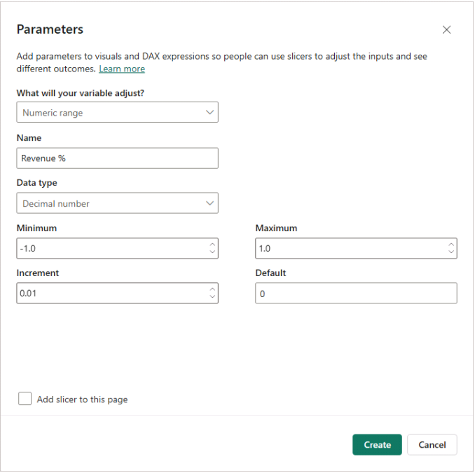
Step 7a. Creating Power BI Parameters for Financial Projections
Financial planning relies on a set of assumptions—revenue growth, cost inflation, payroll increases, capital expenditure, tax rates, debt terms, and more. To keep these inputs flexible, we create What-If parameters so users can adjust assumptions directly from the dashboard.
To get started, go to Modeling → New parameter → Numeric range and define the range, increment, and default value (for example, a Revenue % parameter with −1.0 to +1.0, an increment of 0.01, and a default of 0).
Uncheck Add slicer to this page for now — we’ll place the slicers later when building the forecast dashboard.
For this tutorial, create the following parameters (unless otherwise noted, use Minimum −1.0, Maximum +1.0, Increment 0.01, Default 0):<br />Revenue %, COGS %, Opex %, Salary %, Headcount %, Dep Years (default 5), Tax % (default 0.2), Capex %, Debt Amount, Debt Years, and Debt Interest Annual.
Then, create a few helper measures that reference the selected parameter values. These reusable measures keep the DAX cleaner and also make it easy to override or adjust assumptions later if needed:
Capex % = SELECTEDVALUE ( 'Capex %'[Capex %], 0 )
COGS % = SELECTEDVALUE ( 'COGS %'[COGS %], 0 )
Debt Amount = SELECTEDVALUE ( 'New Debt'[New Debt], 0 )
Debt Interest Annual = SELECTEDVALUE ( 'Debt Interest %'[Debt Interest %], 0 )
Debt Years = SELECTEDVALUE ( 'Debt Period Yrs'[Debt Period Yrs], 0 )
Dep Years = SELECTEDVALUE ( 'Dep Years'[Dep Years], 5 )
Headcount % = SELECTEDVALUE ( 'Headcount %'[Headcount %], 0 )
Opex % = SELECTEDVALUE ( 'Opex %'[Opex %], 0 )
Revenue % = SELECTEDVALUE ( 'Revenue %'[Revenue %], 0 )
Salary % = SELECTEDVALUE ( 'Salary %'[Salary %], 0 )
Tax % = SELECTEDVALUE ( 'Tax %'[Tax %], 0.2 )
Step 7b. Planning the Profit & Loss Forecast
Before forecasting revenue or costs, we need a set of helper measures that define the boundary between actuals and projections. These measures identify the last month of actuals, determine whether the current filter context falls in the actual or forecast period, and mark the start of the forward-looking window.
They form the backbone of nearly every forecasting calculation that follows.
Last Actual Date =
CALCULATE(
    MAX('Calendar'[Date]),
    REMOVEFILTERS('Calendar'),
    'Calendar'[IsActual] = TRUE()
)

Last Actual Year =
YEAR([Last Actual Date])

Last Actual Month =
DATE(
    YEAR([Last Actual Date]),
    MONTH([Last Actual Date]),
    1
)

Is Actual Month =
VAR _this = MIN('Calendar'[MonthStart])
RETURN _this <= [Last Actual Month]

Forecast Start Month =
EDATE([Last Actual Month], 1)
Revenue Forecast Measures
Revenue follows a practical FP&A forecasting method: you start with the average of the last three actual months and then apply the year-on-year Revenue % assumption. The model spreads growth gradually across each forecast year, creating a smooth monthly ramp instead of sudden jumps.
Revenue Base (Last 3 Actual Months Avg) =
VAR _lastActualDate = [Last Actual Date]
VAR _windowStart =
EOMONTH ( _lastActualDate, -3 ) + 1
VAR _total3M =
CALCULATE (
    SUM ( 'pnl_daily_2025'[Amount] ),
    ALL ( 'pnl_daily_2025' ),
    'pnl_daily_2025'[Account] = "Revenue",
    'pnl_daily_2025'[Date] >= _windowStart,
    'pnl_daily_2025'[Date] <= _lastActualDate
)
RETURN
DIVIDE ( _total3M, 3 )

Revenue Forecast (only) =
VAR _g = [Revenue %]
VAR _factor = 1 + _g
VAR _base = [Revenue Base (Last 3 Actual Months Avg)]
VAR _lastActY = [Last Actual Year]
RETURN
SUMX (
    VALUES ( 'Calendar'[MonthStart] ),
    VAR _y = YEAR ( 'Calendar'[MonthStart] )
    VAR _m = MONTH ( 'Calendar'[MonthStart] )
    RETURN
    IF (
        _y <= _lastActY,
        0,
        IF (
            _y = _lastActY + 1,
            _base * ( 1 + _g * _m / 12 ),
            _base
            * ( 1 + _g * _m / 12 )
            * ( _factor ^ ( _y - ( _lastActY + 1 ) ) )
        )
    )
)
COGS Forecast Measures
COGS follows the same FP&A approach as revenue: you take the average of the last three actual months and apply the COGS % assumption year over year. The model phases in the growth gradually across each forecast year to create a smooth monthly cost pattern.
COGS Base (Last 3 Actual Months Avg) =
VAR lastActualDate = [Last Actual Date]
VAR _windowStart =
EOMONTH ( lastActualDate, -3 ) + 1
VAR _total3M =
CALCULATE (
    SUM ( 'pnl_daily_2025'[Amount] ),
    ALL ( 'pnl_daily_2025' ),
    'pnl_daily_2025'[Account] = "COGS",
    'pnl_daily_2025'[Date] >= _windowStart,
    'pnl_daily_2025'[Date] <= lastActualDate
)
RETURN
DIVIDE ( _total3M, 3 )

COGS Forecast (only) =
VAR _g = [COGS %]
VAR _factor = 1 + _g
VAR _base = [COGS Base (Last 3 Actual Months Avg)]
VAR _lastActY = [Last Actual Year]
RETURN
SUMX (
    VALUES ( 'Calendar'[MonthStart] ),
    VAR _y = YEAR ( 'Calendar'[MonthStart] )
    VAR _m = MONTH ( 'Calendar'[MonthStart] )
    RETURN
    IF (
        _y <= _lastActY,
        0,
        IF (
            _y = _lastActY + 1,
            _base * ( 1 + _g * _m / 12 ),
            _base
            * ( 1 + _g * _m / 12 )
            * ( _factor ^ ( _y - ( _lastActY + 1 ) ) )
        )
    )
)
Headcount Forecasting
Headcount planning starts with the last actual month as the base. From there, the model applies the Headcount % year-on-year growth assumption and spreads the increase gradually across the months, creating a smooth and realistic hiring pattern.
The projected values are rounded to whole employees and then used to calculate salary inflation and total payroll cost.
Headcount Base (Dec Actual) =
VAR _lastActualMonthStart = [Last Actual Month]
RETURN
CALCULATE (
    [Headcount (EOP)],
    ALL ( 'Calendar' ),
    'Calendar'[MonthStart] = _lastActualMonthStart
)

Headcount Forecast (only) =
VAR _g        = [Headcount %]
VAR _y        = MAX ( 'Calendar'[Year] )
VAR _m        = MAX ( 'Calendar'[MonthNo] )
VAR _lastActY = [Last Actual Year]
VAR _baseHC   = [Headcount Base (Dec Actual)]
VAR _yearsAfterBudget = _y - ( _lastActY + 1 )
VAR _baseAtYearStart  = _baseHC * POWER ( 1 + _g, _yearsAfterBudget )
VAR _targetForYear    = _baseHC * POWER ( 1 + _g, _yearsAfterBudget + 1 )
VAR _ramp             = _baseAtYearStart + ( _targetForYear - _baseAtYearStart ) * _m / 12
RETURN
IF ( _y > _lastActY, ROUND ( _ramp, 0 ), BLANK() )

Headcount (Actual+Forecast) =
[Headcount (EOP)] + [Headcount Forecast (only)]
Salary and Payroll Forecast Measures
Payroll forecasting combines the projected headcount with salary inflation. The measures first calculate the average salary per employee from the last three actual months, then grow it using the Salary % assumption and multiply it by the forecasted headcount to produce a realistic monthly payroll outlook.
Salary per Head (Base 3M Avg) =
VAR _lastActualDate = [Last Actual Date]
VAR _windowStart = EOMONTH(_lastActualDate, -3) + 1
VAR _totalPayroll3M =
CALCULATE(
    SUM('pnl_daily_2025'[Amount]),
    ALL('pnl_daily_2025'),
    'pnl_daily_2025'[Subcategory] =
    "Payroll (incl. taxes/benefits/bonus accrual)",
    'pnl_daily_2025'[Date] >= _windowStart,
    'pnl_daily_2025'[Date] <= _lastActualDate ) VAR _months3 = CALCULATETABLE( VALUES('Calendar'[MonthStart]), ALL('Calendar'), 'Calendar'[Date] >= _windowStart,
    'Calendar'[Date] <= _lastActualDate
)

VAR _avgHC3M =
AVERAGEX(
    _months3,
    VAR _eop = EOMONTH('Calendar'[MonthStart], 0)
    RETURN
    CALCULATE(
        DISTINCTCOUNT(payroll_roster_2025[EmployeeID]),
        ALL(payroll_roster_2025),
        payroll_roster_2025[HireDate] <= _eop, OR( ISBLANK(payroll_roster_2025[TerminationDate]), payroll_roster_2025[TerminationDate] > _eop
        )
    )
)
VAR _monthlyPayroll = DIVIDE(_totalPayroll3M, 3)
RETURN DIVIDE(_monthlyPayroll, _avgHC3M)

Salary per Head Forecast (only) =
VAR _g        = [Salary %]
VAR _factor   = 1 + _g
VAR _base     = [Salary per Head (Base 3M Avg)]
VAR _y        = MAX ( 'Calendar'[Year] )
VAR _m        = MAX ( 'Calendar'[MonthNo] )
VAR _lastActY = [Last Actual Year]
RETURN
SWITCH (
    TRUE (),
    _y = _lastActY + 1,
    _base * ( 1 + _g * _m / 12 ),
    _y > _lastActY + 1,
    _base
    * ( 1 + _g * _m / 12 )
    * ( _factor ^ ( _y - ( _lastActY + 1 ) ) ),
    BLANK ()
)

Payroll Forecast (only) =
SUMX (
    VALUES ( 'Calendar'[MonthStart] ),
    [Headcount Forecast (only)] * [Salary per Head Forecast (only)]
)
Opex ex Payroll Forecast
The non-payroll operating expense measures follow the same structure: they take a three-month actual average and apply the Opex % growth assumption. They then distribute the increase evenly across each forecast year to maintain a smooth progression of operating costs.
Opex ex Payroll Base (3M Avg) =
VAR _lastActualDate = [Last Actual Date]
VAR _windowStart =
EOMONTH ( _lastActualDate, -3 ) + 1
VAR _total3M =
CALCULATE (
    SUM ( 'pnl_daily_2025'[Amount] ),
    ALL ( 'pnl_daily_2025' ),
    'pnl_daily_2025'[Account] = "Opex",
    'pnl_daily_2025'[Subcategory] <> "Payroll (incl. taxes/benefits/bonus accrual)",
    'pnl_daily_2025'[Date] >= _windowStart,
    'pnl_daily_2025'[Date] <= _lastActualDate
)
RETURN
DIVIDE ( _total3M, 3 )

Opex ex Payroll Forecast (only) =
VAR _g = [Opex %]
VAR _factor = 1 + _g
VAR _base = [Opex ex Payroll Base (3M Avg)]
VAR _lastActY = [Last Actual Year]
RETURN
SUMX (
    VALUES ( 'Calendar'[MonthStart] ),
    VAR _y = YEAR ( 'Calendar'[MonthStart] )
    VAR _m = MONTH ( 'Calendar'[MonthStart] )
    RETURN
    IF (
        _y <= _lastActY,
        0,
        IF (
            _y = _lastActY + 1,
            _base * ( 1 + _g * _m / 12 ),
            _base
            * ( 1 + _g * _m / 12 )
            * ( _factor ^ ( _y - ( _lastActY + 1 ) ) )
        )
    )
)
Step 7c. Forecasting Depreciation Using DAX
Depreciation depends on both existing fixed assets and new capital expenditure. To handle this, the model calculates depreciation in two parts: one based on existing PPE using a fixed 60-month assumption, and another based on forecasted capex using the user-defined Dep Years parameter.
Capex Forecast Measures
The capex measures forecast investment by taking the average monthly investing cash flow from the last actual year and applying the Capex % growth assumption. They produce a smooth forward-looking capex trend that scales naturally with the business instead of relying on fixed manual inputs.
Capex Base (Monthly Avg Last Actual Year) =
VAR _lastActY = [Last Actual Year]
RETURN
AVERAGEX (
    FILTER (
        ALL ( 'cash_flow_monthly_2025' ),
        YEAR ( 'cash_flow_monthly_2025'[Month] ) = _lastActY
        && 'cash_flow_monthly_2025'[Category] = "Investing"
    ),
    'cash_flow_monthly_2025'[Amount]
) * -1

Capex (Forecast Only) =
VAR _lastActY = [Last Actual Year]
VAR _base     = [Capex Base (Monthly Avg Last Actual Year)]
VAR _g        = [Capex %]
VAR _factor   = 1 + _g
RETURN
SUMX (
    VALUES ( 'Calendar'[MonthStart] ),
    VAR _y = YEAR ( 'Calendar'[MonthStart] )
    RETURN
        - SWITCH (
            TRUE(),
            _y > _lastActY, _base * ( _factor ^ ( _y - _lastActY ) ),
            BLANK()
        )
)
Depreciation Forecast Measures
Depreciation measures operate in two parts: they depreciate existing PPE over a fixed 60-month schedule, and they apply the user-defined Dep Years parameter to new forecasted capex. They calculate both components monthly, ensuring depreciation stays aligned with asset additions and remaining useful life.
Existing PPE Depreciation (Forecast Only) =
VAR _depMonths       = 60
VAR _lastActualMonth = [Last Actual Month]
RETURN
    SUMX (
        VALUES ( 'Calendar'[MonthStart] ),
        VAR _curMonth = 'Calendar'[MonthStart]
        RETURN
            IF (
                _curMonth <= _lastActualMonth,
                0,
                VAR _endMonth =
                    MIN (
                        EDATE ( _curMonth, -1 ),
                        _lastActualMonth
                    )
                VAR _startMonth =
                    EDATE ( _curMonth, -_depMonths )
                VAR _capexExistingPool =
                    CALCULATE (
                        SUM ( 'cash_flow_monthly_2025'[Amount] ),
                        ALL ( 'cash_flow_monthly_2025' ),
                        'cash_flow_monthly_2025'[Category] = "Investing",
                        'cash_flow_monthly_2025'[Month] >= _startMonth,
                        'cash_flow_monthly_2025'[Month] <= _endMonth
                    )
                RETURN
                    DIVIDE ( _capexExistingPool, _depMonths )
            )
    )
New Capex Depreciation (Month) =
VAR _depMonths = [Dep Years] * 12
RETURN
SUMX (
    VALUES ( 'Calendar'[MonthStart] ),
    VAR _curMonth = 'Calendar'[MonthStart]
    VAR _startMonth = EDATE ( _curMonth, -_depMonths )
    VAR _endMonth   = EDATE ( _curMonth, -1 )

    -- Rolling depreciation pool
    VAR _capexPool =
        CALCULATE (
            SUMX ( VALUES ( 'Calendar'[MonthStart] ), [Capex (Forecast Only)] ),
            ALL ( 'Calendar' ),
            'Calendar'[MonthStart] >= _startMonth,
            'Calendar'[MonthStart] <= _endMonth
        )
    RETURN
        DIVIDE ( _capexPool, _depMonths )
)
Step 7d. Modeling Debt and Loan Amortisation
To capture financing activity, the model introduces debt forecasting. It assumes a single loan drawn at the start of the forecast period and repaid over the user-selected term.
The model calculates monthly instalments and automatically splits each payment into interest and principal.
As the balance declines, interest costs fall while principal repayment increases, producing a realistic amortisation schedule that feeds directly into projected cash flows and interest expense.
Debt Helper Measures
The debt helper measures establish the structure of the loan forecast. They identify when the debt begins, calculate the total number of repayment months, determine which months fall within the active forecast period, and convert the annual interest rate into its monthly equivalent.
These foundations enable a clean, consistent amortisation schedule.
Debt Start Month =
EDATE ( [Last Actual Month], 1 )

Is Active Debt Forecast Month =
NOT [Is Actual Month]
&& [Debt Amount] <> 0
&& [Debt Years] > 0
&& [Debt Forecast Index] >= 1
&& [Debt Forecast Index] <= [Debt Months]

Debt Forecast Index =
VAR _start = [Debt Start Month]
VAR _this  = MIN('Calendar'[MonthStart])
RETURN
DATEDIFF(_start, _this, MONTH) + 1

Last Actual Debt Balance =
VAR _last = [Last Actual Month]
RETURN
CALCULATE (
    [BS Amount],
    KEEPFILTERS ( DimBS_Category[Category] = "Debt" ),
    'Calendar'[MonthStart] = _last
)

Debt Months = [Debt Years] * 12

Debt Interest Monthly = DIVIDE ( [Debt Interest Annual], 12 )
Debt Calculation Measures
The debt measures apply standard amortisation logic using a Power BI measure equivalent to Excel’s PMT function (external link) to determine monthly payments. They split each payment into interest and principal, update the loan balance accordingly, and add new debt at the start of the forecast.
This produces a realistic month-by-month debt schedule that flows directly into cash flow and interest expense projections.
Debt PMT =
VAR _r = [Debt Interest Monthly]
VAR _n = [Debt Months]
VAR _amt = [Debt Amount]
RETURN
IF (
    _r > 0,
    _amt * _r / (1 - (1 + _r) ^ -_n),
    DIVIDE(_amt, _n)
)

Debt Balance At Period (Forecast) =
VAR _r   = [Debt Interest Monthly]
VAR _k   = [Debt Forecast Index]
VAR _n   = [Debt Months]
VAR _amt = [Debt Amount]
VAR _pmt = [Debt PMT]
VAR _pow = (1 + _r) ^ ( _k - 1 )
RETURN
IF (
    _r > 0,
    _amt * _pow - _pmt * ( (_pow - 1) / _r ),
    _amt - _pmt * (_k - 1)
)

Debt Opening Balance (BoM) =
VAR _actual = IF ( [Is Actual Month], BLANK(), [Last Actual Debt Balance] )
VAR _forecast = IF ( [Is Active Debt Forecast Month], [Debt Balance At Period (Forecast)], 0 )
RETURN
COALESCE(_actual, 0) + _forecast

Debt Draw Amount (Month) =
SUMX(
    VALUES('Calendar'[MonthStart]),
    IF(
        'Calendar'[MonthStart] = [Debt Start Month],
        [Debt Amount],
        0
    )
)

Debt Payment (Month) =
SUMX (
    VALUES('Calendar'[MonthStart]),
    IF ( [Is Active Debt Forecast Month], -[Debt PMT], 0 )
)

Debt Interest Amount (Month) =
VAR _r = [Debt Interest Monthly]
RETURN
SUMX (
    VALUES('Calendar'[MonthStart]),
    VAR _bom = CALCULATE([Debt Opening Balance (BoM)])
    RETURN IF ( _bom = 0, 0, -_bom * _r )
)

Debt Principal Repayment (Month) =
[Debt Payment (Month)] - [Debt Interest Amount (Month)]

Debt Closing Balance (EoM) =
[Debt Opening Balance (BoM)] + [Debt Principal Repayment (Month)]

Debt Balance (Actual+Forecast) =
IF (
    [Is Actual Month],
    CALCULATE (
        [BS Amount],
        KEEPFILTERS ( DimBS_Category[Category] = "Debt" )
    ),
    [Debt Closing Balance (EoM)]
)

Interest Expense (Forecast only) =
IF (SELECTEDVALUE ( 'Calendar'[IsActual] ), 0, [Debt Interest Amount (Month)])
Step 7e. Building Earnings Forecast Measures
With our revenue, COGS, operating expense, payroll, depreciation, and debt interest measures in place, we can now assemble the full Profit and Loss outlook. The earnings measures combine actuals with forward-looking values to produce a complete P&L forecast.
Revenue (Actual+Forecast) = [Revenue] + [Revenue Forecast (only)]

COGS (Actual+Forecast) = [COGS] + [COGS Forecast (only)]

Payroll (Actual+Forecast) = [Payroll Cost] + [Payroll Forecast (only)]

Opex ex Payroll (Actual+Forecast) = [Opex ex Payroll] + [Opex ex Payroll Forecast (only)]

EBITDA (Actual+Forecast) =
[Revenue (Actual+Forecast)] +
[COGS (Actual+Forecast)] +
[Opex ex Payroll (Actual+Forecast)] +
[Payroll (Actual+Forecast)]

Gross Profit (Actual+Forecast) =
[Revenue (Actual+Forecast)] +
[COGS (Actual+Forecast)]

Capex (Actual+Forecast) = [Capex] + [Capex (Forecast Only)]

D&A (Actual+Forecast) =
[D&A] +
(
    [Existing PPE Depreciation (Forecast Only)] +
    [New Capex Depreciation (Month)]
)

EBIT (Actual+Forecast) =
[EBITDA (Actual+Forecast)] + [D&A (Actual+Forecast)]

Income Tax Expense (Forecast only) =
VAR lastActualDate = [Last Actual Date]
RETURN
    SUMX (
        VALUES ( 'Calendar'[MonthStart] ),
        VAR _thisMonth = 'Calendar'[MonthStart]
        VAR _isActual  = _thisMonth <= lastActualDate VAR _pti = [EBIT (Actual+Forecast)] RETURN IF ( NOT _isActual && _pti > 0,
                - _pti * [Tax %],
                0
            )
    )

Income Tax Expense (Actual+Forecast) =
[Income Tax Expense] + [Income Tax Expense (Forecast only)]

Interest Expense (Actual+Forecast) =
[Interest Expense] + [Interest Expense (Forecast only)]

Net Income (Actual+Forecast) =
[EBIT (Actual+Forecast)] +
[Income Tax Expense (Actual+Forecast)] +
[Interest Expense (Actual+Forecast)]
Retained Earnings Forecast
The retained earnings measures start with the last actual closing balance and then accumulate all forward-looking net income from the first forecast month onward. They create a continuous monthly retained earnings trajectory that ties directly to projected profitability and updates dynamically with every scenario change.
Retained Earnings (Actual+Forecast) EOP =
VAR _lastActualMonth = [Last Actual Month]
VAR _thisMonth = MAX ( 'Calendar'[MonthStart] )
VAR _baseRE =
CALCULATE (
    [BS Amount],
    ALL ( 'Calendar' ),
    'Calendar'[MonthStart] = _lastActualMonth
)
VAR _fromFirstForecastMonth = EDATE ( _lastActualMonth, 1 )
VAR _cumNI =
CALCULATE (
    SUMX (
        DATESBETWEEN (
            'Calendar'[MonthStart],
            _fromFirstForecastMonth,
            _thisMonth
        ),
        [Net Income (Actual+Forecast)]
    ),
    ALL ( 'Calendar' )
)
RETURN
IF (
    _thisMonth <= _lastActualMonth,
    [BS Amount],
    _baseRE + _cumNI
)
Step 7f. Creating Cash Flow Forecast Measures
Working capital forecasting is important for producing realistic cash flow projections. The model estimates Accounts Payable and Accounts Receivable based on projected Opex, COGS, and Revenue, applying user-defined ratios for each.
Once the working capital movements are in place, it projects Operating, Investing, and Financing cash flows for both actual and forward-looking periods.
Accounts Payable Forecast Measures
The Accounts Payable measures project AP by applying the Payable % of Opex assumption to forecasted Opex and COGS. They calculate the monthly AP balance, compare each period with the previous one, and derive the working capital movement used in the cash flow forecast.
AP Balance (Actual+Forecast) =
VAR _month          = SELECTEDVALUE('Calendar'[MonthStart])
VAR _lastActualMonth = [Last Actual Month]
VAR _pctPay         = 'Payable % of Opex'[Payable % of Opex Value]
RETURN
IF(
    _month <= _lastActualMonth,
    CALCULATE(
        [BS Amount],
        ALL('Calendar'),
        'Calendar'[MonthStart] = _month
    ),
    VAR _opex =
        CALCULATE(
            [Opex ex Payroll (Actual+Forecast)],
            ALL('Calendar'),
            'Calendar'[MonthStart] = _month
        )
    VAR _cogs =
        CALCULATE(
            [COGS (Actual+Forecast)],
            ALL('Calendar'),
            'Calendar'[MonthStart] = _month
        )
    RETURN
        -(_opex + _cogs) * _pctPay
)

Accounts Payable (Actual+Forecast) EOP =
VAR _lastVisibleMonth = MAX ( 'Calendar'[MonthStart] )
RETURN
CALCULATE (
    [AP Balance (Actual+Forecast)],
    ALL ( 'Calendar' ),
    'Calendar'[MonthStart] = _lastVisibleMonth
)

ΔAccounts Payable (Forecast only) =
VAR _lastActualMonth = [Last Actual Month]
RETURN
SUMX (
    VALUES ( 'Calendar'[MonthStart] ),
    VAR _curMonth = 'Calendar'[MonthStart]
    VAR _isActual = _curMonth <= _lastActualMonth
    VAR _prevMonth = EDATE ( _curMonth, -1 )
    RETURN
    IF (
        _isActual,
        0,
        VAR _apThis =
        CALCULATE (
            [AP Balance (Actual+Forecast)],
            ALL ( 'Calendar' ),
            'Calendar'[MonthStart] = _curMonth
        )
        VAR _apPrev =
        IF (
            _prevMonth <= _lastActualMonth,
            CALCULATE (
                SUM ( balance_sheet_monthly_2025[Amount] ),
                ALL ( balance_sheet_monthly_2025 ),
                balance_sheet_monthly_2025[Category] = "Accounts Payable",
                balance_sheet_monthly_2025[Month] = _prevMonth
            ),
            CALCULATE (
                [AP Balance (Actual+Forecast)],
                ALL ( 'Calendar' ),
                'Calendar'[MonthStart] = _prevMonth
            )
        )
        RETURN _apThis - _apPrev
    )
)
Accounts Receivable Forecast Measures
The Accounts Receivable measures forecast AR by multiplying projected revenue by the Receivable % of Revenue parameter. They calculate the resulting monthly AR balances and use them to compute working capital changes that directly affect operating cash flow.
AR Balance (Actual+Forecast) =
VAR _month = SELECTEDVALUE('Calendar'[MonthStart])
VAR _lastActualMonth = [Last Actual Month]
VAR _pctRec = 'Receivable % of Revenue'[Receivable % of Revenue Value]
RETURN
IF(
    _month <= _lastActualMonth,
    CALCULATE(
        [BS Amount],
        ALL('Calendar'),
        'Calendar'[MonthStart] = _month
    ),
    VAR _rev =
        CALCULATE(
            [Revenue (Actual+Forecast)],
            ALL('Calendar'),
            'Calendar'[MonthStart] = _month
        )
    RETURN
        _pctRec * _rev
)

Accounts Receivable (Actual+Forecast) EOP =
VAR _lastVisibleMonth = MAX ( 'Calendar'[MonthStart] )
RETURN
CALCULATE (
    [AR Balance (Actual+Forecast)],
    ALL ( 'Calendar' ),
    'Calendar'[MonthStart] = _lastVisibleMonth
)

ΔAccounts Receivable (Forecast only) =
VAR _lastActualMonth = [Last Actual Month]
RETURN
SUMX (
    VALUES ( 'Calendar'[MonthStart] ),
    VAR _curMonth = 'Calendar'[MonthStart]
    VAR _isActual = _curMonth <= _lastActualMonth
    VAR _prevMonth = EDATE ( _curMonth, -1 )
    RETURN
    IF (
        _isActual,
        0,
        VAR _arThis =
        CALCULATE (
            [AR Balance (Actual+Forecast)],
            ALL ( 'Calendar' ),
            'Calendar'[MonthStart] = _curMonth
        )
        VAR _arPrev =
        IF (
            _prevMonth <= _lastActualMonth,
            CALCULATE (
                SUM ( balance_sheet_monthly_2025[Amount] ),
                ALL ( balance_sheet_monthly_2025 ),
                balance_sheet_monthly_2025[Category] = "Accounts Receivable",
                balance_sheet_monthly_2025[Month] = _prevMonth
            ),
            CALCULATE (
                [AR Balance (Actual+Forecast)],
                ALL ( 'Calendar' ),
                'Calendar'[MonthStart] = _prevMonth
            )
        )
        RETURN
        _arThis - _arPrev
    )
)
Cash Flow Forecast Measures
The cash flow measures combine operating, investing, and financing activities into a complete monthly projection. They incorporate net income, depreciation, working capital movements, capex, and debt activity to calculate CFO, CFI, CFF, and overall changes in cash for both actual and forward-looking periods.
CFO (Forecast only) =
VAR _lastActualDate = [Last Actual Date]
RETURN
SUMX(
    VALUES('Calendar'[MonthStart]),
    VAR _thisMonth = 'Calendar'[MonthStart]
    RETURN
        IF(
            _thisMonth <= _lastActualDate,
            0,
            [Net Income (Actual+Forecast)]
                - [D&A (Actual+Forecast)]
                - [ΔAccounts Receivable (Forecast only)]
                + [ΔAccounts Payable (Forecast only)]
        )
)

CFI (Forecast only) = [Capex (Forecast Only)]

CFF (Forecast only) =
IF (
    SELECTEDVALUE ( 'Calendar'[IsActual] ),
    0,
    [Debt Draw Amount (Month)]
    + [Debt Principal Repayment (Month)]
)

CFO (Actual+Forecast) = [CFO] + [CFO (Forecast only)]
CFI (Actual+Forecast) = [CFI] + [CFI (Forecast only)]
CFF (Actual+Forecast) = [CFF] + [CFF (Forecast only)]

ΔCash (Actual+Forecast) =
[CFO (Actual+Forecast)] +
[CFI (Actual+Forecast)] +
[CFF (Actual+Forecast)]

CF Amount (Actual+Forecast) =
VAR _cat = SELECTEDVALUE('DimCF_Category'[Category])
VAR _lastActualDate = [Last Actual Date]
RETURN
SUMX(
    VALUES('Calendar'[MonthStart]),
    VAR _thisMonth = 'Calendar'[MonthStart]
    RETURN
        IF(
            _thisMonth <= _lastActualDate,
            [CF Amount],
            SWITCH(
                TRUE(),
                _cat = "Operating", [CFO (Forecast only)],
                _cat = "Investing", [CFI (Forecast only)],
                _cat = "Financing", [CFF (Forecast only)],
                _cat = "Net",
                    [CFO (Forecast only)] + [CFI (Forecast only)] + [CFF (Forecast only)],
                BLANK()
            )
        )
)
Step 7g. Building Balance Sheet Forecast Measures
The final stage of the planning engine combines all previous components—cash flows, working capital, debt balances, depreciation, retained earnings—into complete Balance Sheet projections. These measures provide end-of-period balances, which we will later use for visualising assets, liabilities, and equity across the forecast horizon.
Cash, Capital, and Fixed Assets Forecast Measures
These measures bring together the core building blocks of the model to project cash, paid-in capital, and net fixed assets. They derive cash by cumulatively summing operating, investing, and financing cash flows, keep paid-in capital fixed after the last actual month, and update net PPE each period based on capex and depreciation activity.
Cash (Actual+Forecast) EOP =
VAR _firstMonth =
CALCULATE (
    MIN ( 'Calendar'[MonthStart] ),
    ALL ( 'Calendar' ),
    'Calendar'[IsActual]
)
VAR _thisMonth =
MAX ( 'Calendar'[MonthStart] )
VAR _openingCashAtStart = 0
VAR _cumuDelta =
CALCULATE (
    SUMX (
        DATESBETWEEN (
            'Calendar'[MonthStart],
            _firstMonth,
            _thisMonth
        ),
        [ΔCash (Actual+Forecast)]
    ),
    ALL ( 'Calendar' )
)
RETURN
_openingCashAtStart + _cumuDelta

Paid-in Capital (Actual+Forecast) EOP =
VAR _month = MAX('Calendar'[MonthStart])
VAR _last  = [Last Actual Month]
RETURN
IF(
    _month <= _last,
    [BS Amount],
    CALCULATE(
        [BS Amount],
        ALL('Calendar'),
        'Calendar'[MonthStart] = _last
    )
)

Net PPE (Actual+Forecast) EOP =
VAR _lastActualMonth = [Last Actual Month]
VAR _thisMonth = MAX ( 'Calendar'[MonthStart] )
VAR _fromFirstForecastMonth = [Forecast Start Month]
VAR _basePPE =
CALCULATE (
    [BS Amount],
    ALL ( 'Calendar' ),
    'Calendar'[MonthStart] = _lastActualMonth
)
VAR _cumChange =
CALCULATE (
    SUMX (
        DATESBETWEEN (
            'Calendar'[MonthStart],
            _fromFirstForecastMonth,
            _thisMonth
        ),
        - [Capex]
        - [Capex (Forecast Only)]
        + [Existing PPE Depreciation (Forecast Only)]
        + [New Capex Depreciation (Month)]
    ),
    ALL ( 'Calendar' )
)
RETURN
IF (
    _thisMonth <= _lastActualMonth,
    [BS Amount],
    _basePPE + _cumChange
)
Balance Sheet Forecast Measures
The final balance sheet measures translate all forecast logic into category-level values for reporting. They calculate each major balance sheet line—cash, debt, receivables, payables, PPE, capital, and retained earnings—using its corresponding forecast logic.
Together, these measures produce a complete and dynamic projected balance sheet for every month.
BS Amount (Last Actual EOP) =
VAR _lastActualMonth = [Last Actual Month]
RETURN
CALCULATE (
    [BS Amount],
    ALL ( 'Calendar' ),
    'Calendar'[MonthStart] = _lastActualMonth
)

BS Amount (Actual+Forecast – per Category) =
VAR cat =
SELECTEDVALUE (DimBS_Category[Category])
RETURN
SWITCH (
    TRUE (),
    cat = "Cash",                        [Cash (Actual+Forecast) EOP],
    cat = "Net PPE",                     [Net PPE (Actual+Forecast) EOP],
    cat = "Debt",                        [Debt Balance (Actual+Forecast)],
    cat = "Accounts Receivable",         [Accounts Receivable (Actual+Forecast) EOP],
    cat = "Accounts Payable",            [Accounts Payable (Actual+Forecast) EOP],
    cat = "Paid-in Capital",             [Paid-in Capital (Actual+Forecast) EOP],
    cat = "Retained Earnings",           [Retained Earnings (Actual+Forecast) EOP],
    BLANK ()
)

BS Amount (Actual+Forecast) =
IF (
    HASONEVALUE ( DimBS_Category[Category] ),
    [BS Amount (Actual+Forecast – per Category)],
    SUMX (
        VALUES ( DimBS_Category[Category] ),
        [BS Amount (Actual+Forecast – per Category)]
    )
)
Step 8. Building a Financial Planning & Forecast Dashboard
With the forecasting measures complete, you can move into the visualisation phase and begin assembling the financial planning dashboard. This step turns the forecasting logic into an interactive, user-friendly Power BI report.
You’ll start by building a profit and loss forecast driven by the parameters created earlier, then expand the dashboard with cash flow forecasting, debt amortisation, and balance sheet projections.
Each page will respond instantly to assumption changes, giving you a flexible and dynamic planning environment.
Step 8a. Building the Profit & Loss Forecast Dashboard
Profit and Loss Forecast
This page presents the projected profit and loss statement, where revenue, operating expenses, payroll, depreciation, interest, and tax all respond dynamically to parameter adjustments. It forms the core of the planning dashboard and lets you explore how growth assumptions flow through the financials.
Parameters
Begin by placing the key P&L-related parameters on the page. Insert a slicer and select your first parameter field, such as ‘Revenue %’[Revenue %]. Format it as a percentage and update the slicer title in the Format pane so its purpose is immediately clear. Repeat this process for COGS %, Opex %, Salary %, Headcount %, Tax %, and Dep Years, formatting each slicer according to its input type.
Next, add a slicer using Calendar[Year] to provide a convenient page-level filter, and switch it to a dropdown for a cleaner layout.
Finally, open the Filter pane and add Calendar[IsForecast] to Filters on this page, setting it to True so the dashboard displays only the forecast period.
Monthly Profit and Loss Forecast
This matrix displays the full monthly P&L, giving you a clear view of how revenue, margins, costs, and net income evolve throughout the forecast period.
Insert a Matrix visual and place Calendar[Year] at the top of the Rows, with Calendar[MonthStart] beneath it. Add the following measures to the Values: Revenue (Actual+Forecast), COGS (Actual+Forecast), Gross Profit (Actual+Forecast), Opex ex Payroll (Actual+Forecast), Payroll (Actual+Forecast), D&A (Actual+Forecast), Income Tax Expense (Actual+Forecast), Interest Expense (Actual+Forecast), and Net Income (Actual+Forecast).
Rename fields for readability, format MonthStart as yyyy-mm, and refine headers and titles in the Format pane for a clean final layout.

Annual P&L Graph
This visual provides a high-level, year-by-year summary of the business by combining revenue, costs, and payroll with headcount projections. It helps you spot margin trends and efficiency changes much more easily.
To build the Annual P&L Graph, insert a Line and Clustered Column chart and set Calendar[Year] as the X-axis. Assign Revenue (Actual+Forecast), COGS (Actual+Forecast), Opex ex Payroll (Actual+Forecast), and Payroll (Actual+Forecast) to the column portion of the visual, then place Headcount Forecast on the line axis.
Once the measures are in place, refine the titles, legend, and formatting in the Format pane to create a clean and informative annual P&L view.
Annual P&L Summary
To complement the monthly and graphical P&L views, this page includes an annual summary that aggregates projected financials at the year level — ideal for presentations or executive review. Insert another Matrix visual and place Calendar[Year] in the Rows, then add the key measures — Revenue (Actual+Forecast), COGS (Actual+Forecast), Gross Profit (Actual+Forecast), EBITDA (Actual+Forecast), and Net Income (Actual+Forecast) — to the Values.
Format the headers and rename fields where needed to keep the layout clear and readable.
Note: To ensure the monthly matrix remains responsive to the Year slicer while the annual summary stays independent, open Format → Edit interactions and set the annual visuals to ignore the slicer.
Step 8b. Cash Flow, Debt & Balance Sheet Forecast Dashboard
With the P&L forecast complete, the next page brings together operating cash flow, investing activity, financing flows, and the resulting balance sheet projections. This part of the dashboard uses a separate set of parameters tied to debt, capex, and working-capital assumptions, giving you full control over the financial forecast.
Parameters
Begin by adding the parameters that control cash flow and financing activity. Insert a slicer for New Debt and format it as a currency field. Then, repeat the process for Debt Interest %, Debt Period Yrs, Capex %, Receivable % of Revenue, and Payable % of Opex.
Use the Format pane to label each slicer clearly so users understand how these assumptions feed into the forecast.
Cash Flow Forecast
Next, add the cash flow forecast visual, which displays operating, investing, and financing flows together with the resulting net cash movement across the forecast period. Insert a Matrix and place Calendar[Year] in the Columns—adding quarters or months beneath it if you want expandable detail.
In the Rows, use DimCF_Category[Category], and add CF Amount (Actual+Forecast) to the Values.
Finish by formatting the headers and number display to keep the layout clear and easy to read.
Annual Debt Schedule
The debt schedule provides a year-by-year view of opening balances, new borrowings, principal repayments, closing balances, and interest expense — all driven by your debt parameters.
Insert another Matrix visual and place Calendar[Year] in the Rows. Add the key measures — Debt Opening Balance (BoM), Debt Draw Amount (Month), Debt Principal Repayment (Month), Debt Closing Balance (EoM), and Debt Interest Amount (Month) — to the Values.
Finally, format the column headers and labels so the schedule aligns with the rest of the dashboard.
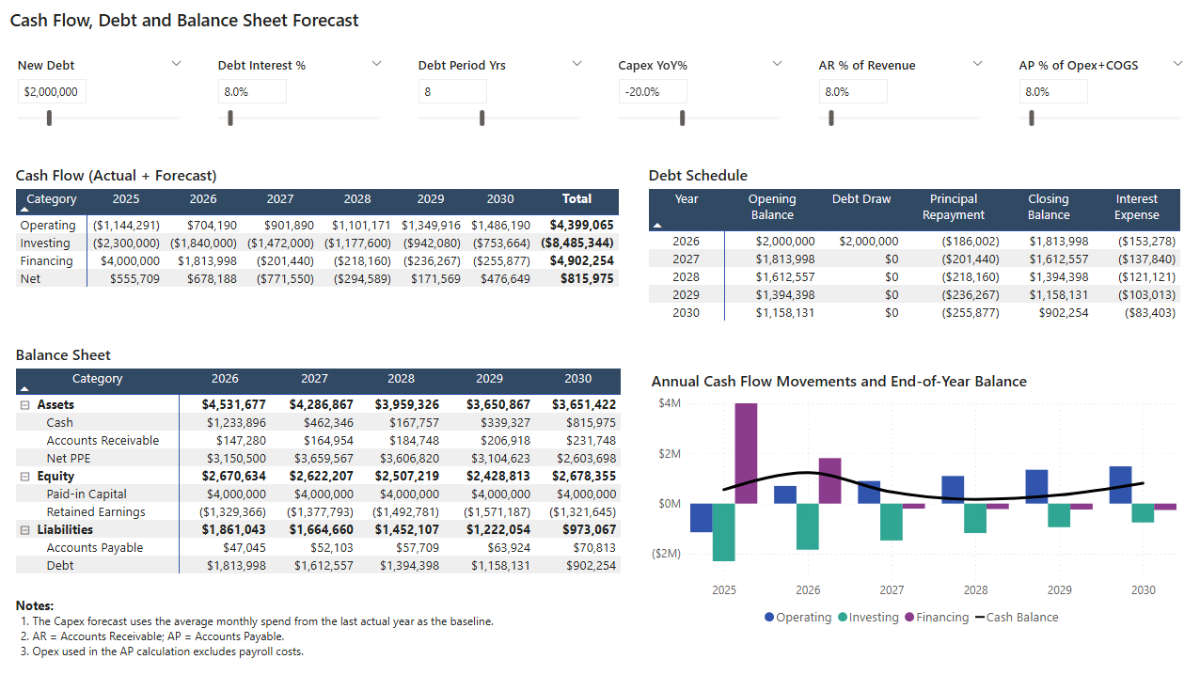
Balance Sheet Forecast
Now create the balance sheet view, which presents projected assets, liabilities, and equity for each forecast year. Insert a Matrix and place Calendar[Year] in the Columns. In the Rows, add DimBS_Category[Section] followed by DimBS_Category[Category], and use BS Amount (Actual+Forecast) as the Value.
If you prefer a cleaner display, you can rename Section to “Category” and Category to “SubCategory.”
Finish by formatting the column headers to match the rest of your report style.
Annual Cash Flow Movement and Ending Balance
To illustrate liquidity trends across the forecast horizon, add a combined visual that shows operating, investing, and financing flows alongside the resulting year-end cash balance.
Insert a Line and Clustered Column chart and use Calendar[Year] for the X-axis. Assign CFO (Actual+Forecast), CFI (Actual+Forecast), and CFF (Actual+Forecast) to the column portion of the chart, then place Cash (Actual+Forecast) EOP on the line axis.
Once the measures are in place, refine the titles, legend, and styling to complete the visual.
Step 8c. Syncing Power BI Filters and Forecast Parameters
Because the forecast spans two pages, it’s important to keep all parameters synchronised so that any change on one page updates the other automatically. Power BI’s Sync Slicers pane gives you full control over this behaviour.
Select any parameter slicer and open the Sync slicers pane. You’ll see a table listing each report page with options to sync the slicer and control its visibility. Parameters driving the P&L — such as revenue and cost growth — should remain visible only on the P&L page but sync with the Cash Flow/Debt page so both views use the same assumptions.
Likewise, debt- and capex-related parameters should appear only on the cash flow page while still synchronising with the P&L page to keep the forecast aligned.
Step 8d. Scenario Testing and Sensitivity Analysis
With the planning dashboard complete, you can now explore how different combinations of assumptions influence financial performance. Scenario testing allows you to adjust multiple parameters at once to model coherent economic conditions—such as inflation shocks or accelerated growth—while sensitivity analysis isolates a single variable to understand its specific impact on profitability, liquidity, or leverage.
Suggested what-if scenarios:
- Scenario #0 – Base case: No changes to revenues or costs, no debt, default tax settings, and standard working-capital assumptions.
- Scenario #1 – Moderate growth: Increased revenue and cost assumptions with debt financing enabled, similar to the examples shown in your dashboard preview.
- Scenario #2 – Inflationary pressure: Higher interest rates combined with elevated operating costs.
- Scenario #3 – Growth scenario: Strong revenue expansion paired with lower interest rates to reflect favourable market conditions.
📌 Recap: Building a Financial Planning & Analysis Dashboard in Microsoft Power BI
Here’s a quick recap of the steps we followed to build a complete financial planning and analysis (FP&A) dashboard in Microsoft Power BI:
- Load and explore the financial data. We imported daily P&L entries, monthly balance sheet and cash flow data, and a payroll roster, then previewed each table to understand revenue, expenses, headcount, and cash movements.
- Create a dynamic calendar table. We built a DAX-driven Calendar table covering all historical activity and five future forecast years, then marked it as the official date table.
- Model the data into a star-schema. We created P&L, cash flow, and balance sheet category dimensions, added payroll and department lookup tables, and connected everything to Calendar for clean financial reporting.
- Build foundational actuals measures. We defined the core Actuals logic for Revenue, COGS, Operating Expenses, Payroll, D&A, Interest, Net Income, Balance Sheet accounts, and Cash Flow movements.
- Create What-If Parameters and Forecast DAX. We added YoY growth assumptions and built forward-looking measures for revenue, operating expenses, payroll inflation, headcount, capex, depreciation, debt, working capital, and net cash flow.
- Build the Profit & Loss Forecast page. We combined slicers, a monthly P&L matrix, an annual summary matrix, and a line/column chart to visualize the projected P&L under different scenarios.
- Build the Cash Flow, Debt & Balance Sheet Forecast page. We added cash flow forecasts, debt amortisation schedules, balance sheet projections, and annual cash movement visuals — all driven by parameters.
- Sync slicers and run scenario testing. We synchronised parameters across pages and used scenario combinations (inflation, growth, interest rate shocks) to test the model’s sensitivity.
By following these steps, you now have a full Power BI FP&A model capable of projecting a complete three-statement forecast with dynamic assumptions.
🔎 Preview the Interactive Financial Planning & Analysis Dashboard
Explore the finished FP&A dashboard — the same build from this tutorial. Adjust revenue growth, cost inflation, payroll parameters, capex, debt terms, and working capital assumptions, and watch the P&L, cash flow, and balance sheet update instantly.
📥 Download My Financial Planning & Analysis Dashboard Template
To help you get started quickly, I’ve prepared a ready-to-use Power BI package that includes:
- Power BI (.pbix) file with all actuals & forecast logic, parameters, and dashboard pages.
- CSV files for the P&L, balance sheet, cash flow, payroll, and calendar data used in the model.
- A complete DAX file containing all real measures grouped exactly as structured in this tutorial.
This template lets you build a full FP&A forecast, evaluate financial performance, and test multiple planning scenarios with ease.
Secure Checkout | Instant Download | 30-Day Money-Back Guarantee
Secure Checkout | Instant Download | 30-Day Money-Back Guarantee
Video Tutorial on Building a Power BI FP&A Dashboard
My complete video tutorial explains how to build and customize a Financial Planning & Analysis (FP&A) dashboard in Microsoft Power BI, covering budgeting, forecasting, cash flow planning, and debt modeling.
In the video, you’ll learn:
- How to load and structure your data model, including a Calendar table and supporting DAX tables.
- How to write core DAX financial measures for P&L, Cash Flow, and Balance Sheet reporting.
- How to visualise and analyse actual financial performance with interactive Power BI dashboards.
- How to use parameters and DAX logic to build scenario-based P&L forecasts and planning.
- How to forecast cash, balance sheet movements, and model debt schedules in Power BI.
By the end of the tutorial, you’ll know how to build an end-to-end Power BI FP&A dashboard that supports analysis, planning, and debt forecasting in one integrated model.

Get in Touch
 Hi, I’m Jacek. I’m passionate about Microsoft Power BI, DAX, and financial analytics.
I hope this tutorial helped you build a complete FP&A model with a dynamic forecast across the P&L, cash flow, and balance sheet.
If you’d like support with forecasting, scenario modeling, or financial dashboards, feel free to get in touch.
You can also explore more step-by-step tutorials, or check out my One-to-One Training and Data Analytics Support if you’d like personalised guidance.
Disclaimer: This tutorial is for informational and educational purposes only and should not be considered professional advice.
Explore More Tutorials
-
- Power BI Sales Analysis & Forecast Dashboard Tutorial — Build a complete sales and margin analysis model, including clean DAX, what-if parameters, and dynamic revenue forecasting.
- Power BI Consolidated P&L Forecast Tutorial — Create a multi-entity profit & loss model using a structured data schema, transparent DAX, and a full set of financial reporting dashboards.
- Power BI Project Planning & Cost Management Dashboard Tutorial — Build a complete project planning model covering project timelines, resources, and scenario-based sensitivity testing.
- Power BI Project Financing and Revenue Recognition Tutorial — Learn about creating revenue recognition, debt forecasting, cash flow, returns, and credit metrics dashboard.
- Excel Cash Flow Forecast Tutorial — Build a rolling 3-statement cash flow forecast in Microsoft Excel, connecting revenue, expenses, working capital, and financing activity into one model.