How to Build a Project Finance and Revenue Recognition Dashboard in Microsoft Power BI

Last Updated on January 2, 2026

This tutorial shows how to build a project finance and revenue recognition model in Microsoft Power BI using projects, contracts, CAPEX, and billing data. The model focuses on how capital investment, contract value, and cash flows evolve over time in long-lived projects, where costs are incurred before revenue is fully realized.

We’ll load and validate the data, create a proper Calendar table and relationships, and then build the DAX measures that power the model. DAX is where the financial logic lives in this tutorial: it turns raw tables into reusable measures for revenue recognition (milestone vs service), contract assets and liabilities, and time-based views that remain consistent as you filter by project, contract, or customer.

Finally, we’ll layer in project financing—including debt calculation, a dynamic debt forecast, interest expense, and levered vs unlevered cash flows—then finish with What-If parameters for structured scenario testing. You can download the finished Power BI file or preview the interactive dashboard at the end to follow along.

Note: The examples used throughout are intentionally simplified and illustrative, focusing on modelling structure and DAX design rather than formal accounting guidance. They are meant to show practical patterns for building project finance and revenue recognition logic in Microsoft Power BI, not to prescribe accounting treatment for specific projects.

Step 1. Load and Review Project Finance Data in Microsoft Power BI

In this first step, we load the core project finance and revenue datasets into Microsoft Power BI and validate the key fields before building any relationships or DAX measures. The goal here is not transformation or optimisation. Instead, we ensure the data is structurally sound and ready for time-based analysis later in the model.

The example data represents a telecom infrastructure operator delivering network assets such as fibre builds, towers, and small cells under long-term customer contracts. The datasets are designed to illustrate how CAPEX, contracts, billing, and revenue recognition interact over time, especially in projects where construction spend ramps up first and contractual revenue follows later.

Although the scenario is telecom-based, the data model and logic are intentionally generic and apply to any capital-intensive project where financing decisions depend on project progress rather than static budgets.

1.1 Import and Review Project, Contract, CAPEX, and Billing Tables

Open Microsoft Power BI Desktop and load each CSV file so we can review the structure before building the data model or writing any DAX measures. At this stage, we are only interested in understanding what each table represents and how it will later contribute to project finance and revenue recognition analysis.

From Home → Get Data → Text/CSV, import the following datasets included with this tutorial:

• dim_projects — Defines the list of construction projects and key milestones such as Ready for Service (RFS). These dates later drive milestone-based revenue recognition and the start of financing repayment logic.
• dim_contracts — Stores customer contracts linked to each project, including contract start and end dates, total transaction value, and the allocation between milestone revenue and recurring service revenue.
• fct_capex — Contains monthly forecast CAPEX by project. These values drive construction cash outflows, debt draw calculations, cumulative invested capital, and equity funding analysis.
• fct_billing — Records customer billing events (invoices) over time. Billing is intentionally kept separate from revenue recognition so that contract assets and contract liabilities arising from timing differences can be analysed explicitly.

1.2 Validate Data Types for Time and Financial Analysis

Once the files are loaded, open each query in Power Query and review the column data types. This step is easy to overlook, but it is critical for reliable DAX calculations later—especially for time intelligence, revenue recognition logic, and project finance measures.

All date-related fields, including project milestones, contract start and end dates, invoice dates, and monthly CAPEX periods, should be set to Date rather than Date/Time. This ensures that the Calendar table can filter these fields consistently and that time-based calculations behave as expected.

Financial and percentage fields should be stored as Decimal Number values. Amounts such as CAPEX, budgets, and contract values should remain numeric, while percentage fields—such as milestone and service allocations—should be expressed as decimals (for example, 0.25 for 25%). Using whole numbers for percentages will silently distort revenue recognition and financing calculations later in the model.

At this stage, no transformations are required beyond data type validation. Before closing Power Query, take a moment to sanity-check the data: confirm that row counts look reasonable, key fields are populated where expected, and project timelines align with the underlying scenario.

Once you are comfortable with the structure, select Close & Apply to load the data into the model.

Step 2. Build the Calendar Table and Data Model

At this point, the data is loaded but not yet usable for meaningful analysis. Before we create any revenue recognition, debt calculation, or project finance DAX measures, we need two foundations in place: a proper Calendar table and a clean, well-defined data model.

The Calendar table provides a single, consistent time axis across projects, contracts, CAPEX, billing, and financing. It underpins all time-based analysis in the model. The data model then defines how these tables relate to each other so that filters flow correctly by project, contract, customer, and time.

2.1 Create a Calendar Table for Revenue and Financing Analysis

Create a new table using DAX and name it Calendar. This table will act as the single time axis for the entire model and will control all time-based calculations later in the tutorial, including revenue recognition, debt forecast, interest expense, and cash-flow analysis.

The DAX below builds the Calendar dynamically by scanning all relevant date columns in the model and finding the earliest and latest dates needed. This avoids hardcoding boundaries and ensures the Calendar always covers the full project and contract lifecycle present in the data.

In practical terms, CALENDAR generates the date range, and ADDCOLUMNS adds the Year, Quarter, and Year-Month attributes you will use in visuals and in DAX measures. Those derived columns also help keep charts and tables sorted correctly when you analyse project revenue, CAPEX, and financing over time.

Calendar = 
VAR MinDate =
    MINX (
        UNION (
            SELECTCOLUMNS ( fct_capex,     "Date", fct_capex[MonthStart] ),
            SELECTCOLUMNS ( fct_billing,   "Date", fct_billing[InvoiceDate] ),
            SELECTCOLUMNS ( dim_projects,  "Date", dim_projects[RFSDate] ),
            SELECTCOLUMNS ( dim_contracts, "Date", dim_contracts[ContractStart] ),
            SELECTCOLUMNS ( dim_contracts, "Date", dim_contracts[ContractEnd] )
        ),
        [Date]
    )
VAR MaxDate =
    MAXX (
        UNION (
            SELECTCOLUMNS ( fct_capex,     "Date", fct_capex[MonthStart] ),
            SELECTCOLUMNS ( fct_billing,   "Date", fct_billing[InvoiceDate] ),
            SELECTCOLUMNS ( dim_projects,  "Date", dim_projects[RFSDate] ),
            SELECTCOLUMNS ( dim_contracts, "Date", dim_contracts[ContractStart] ),
            SELECTCOLUMNS ( dim_contracts, "Date", dim_contracts[ContractEnd] )
        ),
        [Date]
    )
RETURN
ADDCOLUMNS (
    CALENDAR ( MinDate, MaxDate ),
    "Year", YEAR ( [Date] ),
    "QuarterNumber", QUARTER ( [Date] ),
    "Quarter", "Q" & QUARTER ( [Date] ),
    "MonthNumber", MONTH ( [Date] ),
    "YearMonth", FORMAT ( [Date], "YYYY-MM" ),
    "MonthStart", DATE ( YEAR ( [Date] ), MONTH ( [Date] ), 1 )
)

After the table is created, sort Quarter by QuarterNumber and sort YearMonth by MonthStart so visuals display in the correct chronological order.

Once that is done, mark the table as a Date table using the Date column (Modeling → Mark as date table). This ensures time intelligence functions behave correctly and prevents Microsoft Power BI from creating hidden, auto-generated date tables in the background.

2.2 Define Relationships Between Projects, Contracts, and Time

With the Calendar table in place, the next step is to define the relationships that tie projects, contracts, CAPEX, billing, and time into a single analytical model. As with any financial model in Microsoft Power BI, the goal is clarity and predictability: one-to-many relationships, single-direction filtering, and no ambiguity in how filters propagate.

Create the following relationships in Model view, using cardinality 1:* and single-direction filtering throughout.

Model Relationships (Cardinality: 1:*, Direction: Single)

Calendar relationships

• Calendar[Date] → fct_capex[MonthStart]
• Calendar[Date] → fct_billing[InvoiceDate]

Project and contract relationships

• dim_projects[ProjectID] → fct_capex[ProjectID]
• dim_projects[ProjectID] → dim_contracts[ProjectID]
• dim_contracts[ContractID] → fct_billing[ContractID]

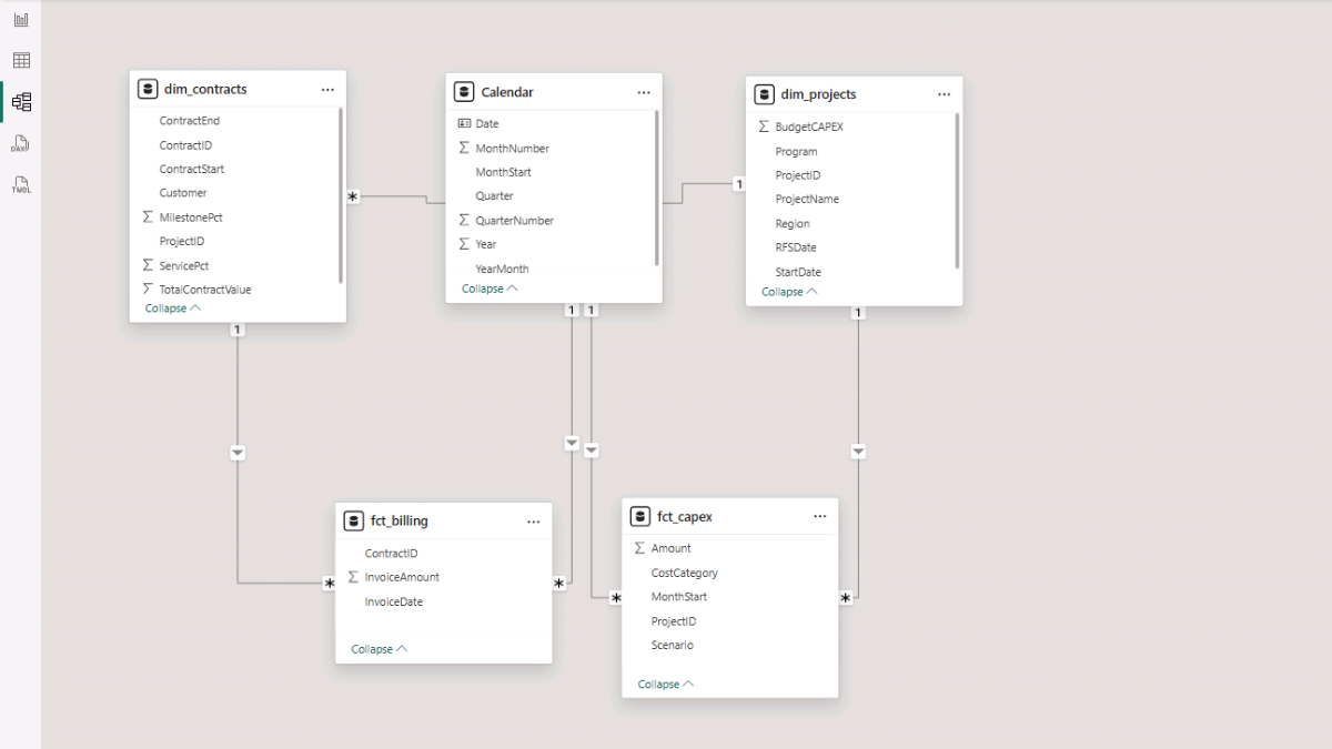
This structure ensures that time filters from the Calendar table apply consistently across CAPEX and billing, construction costs roll up correctly by project, and customer billing remains tied to the correct contract and project context. It also provides a stable foundation for revenue recognition, debt forecast, and cash-flow calculations introduced in later steps.

Step 3. Create Core DAX Measures for CAPEX and Contract Values

With the Calendar table and data model in place, we can now define the core DAX measures that drive the entire dashboard. Measures are reusable calculations that evaluate dynamically based on filter context, allowing the same logic to work consistently across projects, customers, and time periods.

In this step, the logic is intentionally simple. The objective is to establish reliable base measures for CAPEX and contract values that will be reused later for revenue recognition, debt calculation, debt forecasting, and cash-flow analysis.

To keep the file organised as the number of measures grows—especially once scenario logic is added later—all DAX measures in this tutorial are stored in a dedicated measures table.

In Power BI Desktop, go to Home → Enter Data, name the table Measures_Table, and click Load. For each calculation below, right-click Measures_Table and choose New measure.

To improve readability and maintainability, assign measures to logical subfolders using the Display folder property in Model view. Grouping measures by topic (for example: Revenue, Financing, Cash Flow, Valuation, Credit Metrics) makes the model easier to navigate as it scales.

3.1 CAPEX DAX Measures (Forecast vs Budget)

We start with CAPEX, as it anchors the construction timeline and later determines financing needs. These measures focus on forecast CAPEX, cumulative investment over time, and comparison against the original project budget.

CAPEX Amount

This base measure simply aggregates monthly CAPEX amounts from the fact table. It serves as the foundation for all other CAPEX-related calculations.

CAPEX Amount :=
SUM ( fct_capex[Amount] )

Project CAPEX (Forecast)

This measure isolates forecast CAPEX only. CALCULATE is used to modify the filter context so that the same underlying CAPEX data can be reused for different scenarios without duplicating logic.

Project CAPEX (Forecast) :=
CALCULATE ( [CAPEX Amount], fct_capex[Scenario] = "Forecast" )

Project CAPEX Cumulative Forecast

Accumulates forecast CAPEX over time up to the selected month. It uses a common DAX pattern for cumulative totals: iterating over the Calendar table and summing monthly values up to the current point in time.

Project CAPEX Cumulative Forecast =
VAR AsOfMonth = MAX ( Calendar[MonthStart] )
RETURN
SUMX (
    FILTER ( ALL ( 'Calendar' ), Calendar[MonthStart] <= AsOfMonth ),
    CALCULATE ( [Project CAPEX (Forecast)] )
)

Project CAPEX Budget

Aggregates the total budgeted CAPEX defined at the project level. Unlike forecast CAPEX, the budget is static and does not vary by month.

Project CAPEX Budget :=
SUM ( dim_projects[BudgetCAPEX] )

Project CAPEX Variance to Budget (Forecast)

Compares cumulative forecast CAPEX against the original project budget, highlighting whether the project is trending over or under budget.

Project CAPEX Variance to Budget (Forecast) =
[Project CAPEX Cumulative Forecast] - [Project CAPEX Budget]

3.2 Contract Value and Allocation Measures

Next, we define measures that describe the commercial value of projects through their customer contracts. These measures are essential for revenue recognition, as they determine how much value is recognized at milestones versus spread over the service period.

Project Transaction Price

Sums the total transaction value across all contracts in the current filter context. It represents the total contracted revenue associated with the selected projects.

Project Transaction Price :=
SUM ( dim_contracts[TotalContractValue] )

Project Milestone Allocation

Calculates the portion of the transaction price allocated to milestone revenue. SUMX is used to evaluate each contract individually and apply its milestone percentage before summing the results.

Project Milestone Allocation :=
SUMX (
    dim_contracts,
    dim_contracts[TotalContractValue] * dim_contracts[MilestonePct]
)

Project Service Allocation

Calculates the portion of contract value allocated to recurring service revenue. Like the milestone allocation, it iterates contract by contract so different allocation percentages are handled correctly.

Project Service Allocation :=
SUMX (
    dim_contracts,
    dim_contracts[TotalContractValue] * dim_contracts[ServicePct]
)

Projects Count

This simple measure counts distinct projects in the current filter context and is mainly used for summary cards and high-level portfolio views.

Projects Count :=
DISTINCTCOUNT ( dim_projects[ProjectID] )

Step 4. Build the Core Power BI Report Pages

With the core DAX measures in place, we can now start building the report pages that turn the model into a usable Power BI dashboard. In this step, we focus on two pages: a high-level Projects Overview and a more detailed Projects Detail page.

At this stage, the visuals are intentionally descriptive rather than analytical. Their purpose is to validate that CAPEX, contract values, billing, and timelines behave as expected before introducing revenue recognition and project finance logic in later steps.

4.1 Projects Overview

The Projects Overview page provides a portfolio-level snapshot across all projects. It answers basic but essential questions: how many projects are active, how much capital is being invested, and how contract value compares to construction cost.

a. Key Project Metrics

We start with headline metrics shown as cards.

Go to Report view → Home → Visuals gallery and insert a Card (new) visual. Add the following measures to the Data field: Projects Count, Project CAPEX (Forecast), Project Transaction Price, Project Milestone Allocation, Project Service Allocation

Right-click each field name and select Rename for this visual to adjust labels. Use the Format pane to control layout, background, callout values, and font colours so the cards read cleanly as portfolio KPIs.

b. Project Contract Value vs CAPEX

This chart compares commercial value against construction cost at the individual project level and helps identify projects where CAPEX is high relative to contract value.

Insert a Clustered bar chart from the Visuals gallery. Add Project Name to the axis, and add Project Transaction Price and Project CAPEX (Forecast) as values.

Rename the measures for clarity and remove axis titles from the Format pane to keep the visual clean. Adjust the legend and title formatting as needed.

c. Total Contract Value by Customer

This visual shifts the focus from projects to customers and highlights revenue concentration across the customer base.

Insert a Treemap visual. Add Customer to Category and Total Contract Value to Values. In the Format pane, enable Data labels so relative sizes are easy to interpret.

d. Monthly Billing

This chart shows invoicing activity over time. At this stage, billing is shown independently of revenue recognition to reinforce that invoices and accounting revenue follow different timing.

Insert a Clustered column chart. Add Calendar[MonthStart] to the X-axis and Invoice Amount to the Y-axis. Remove axis titles and adjust the chart title formatting from the Format pane.

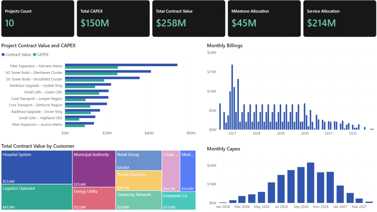
e. Monthly CAPEX

This visual shows how construction spend ramps up and down over time. Later, this same pattern will drive debt drawdowns and cumulative investment.

Reuse a Clustered column chart. Add Calendar[MonthStart] to the X-axis and Project CAPEX (Forecast) to the Y-axis. Apply the same formatting conventions used for Monthly Billing to keep visuals consistent.

4.2 Projects Detail

The Projects Detail page provides a more granular view, combining project, contract, timeline, and value information into a single table. This page is especially useful for validation and ad-hoc analysis.

a. Project and Contract Summary Table

This table brings together descriptive project attributes, contract timelines, and value allocations so you can verify that everything lines up correctly before layering in revenue recognition and financing logic.

Go to Report view → Home → Visuals gallery and insert a Table visual. Add the following fields to the Columns well: Project Name, Contract ID, Customer, RFS Date, Contract Start, Contract End, Budget CAPEX, Total Contract Value, Project Milestone Allocation, Project Service Allocation

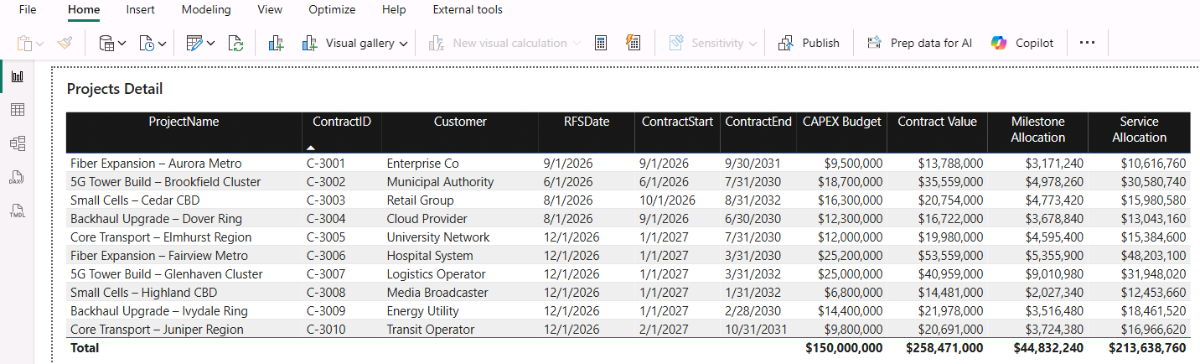
Rename columns where needed for readability and use the Format pane to adjust column headers, gridlines, background colour, and font settings.

Step 5. Revenue Recognition (Milestone and Service)

In this step, we introduce revenue recognition logic and separate it clearly from billing. This distinction is fundamental in project finance and long-term contract analysis. Invoices represent cash timing, while revenue recognition reflects economic performance.

We follow standard accounting principles (external link), but implement them in a practical, Power BI–friendly way. Milestone revenue is recognized at a specific point in time, typically when a project reaches Ready for Service (RFS). Service revenue is recognized evenly over the contract period. Together, these measures allow us to analyse project revenue, contract positions, and timing differences that later affect cash flow and financing.

5.1 Milestone and Service Revenue Measures

Project Revenue Recognized (Milestone, Cumulative)

Recognizes milestone revenue once a project reaches its Ready for Service (RFS) date. For each contract, the milestone portion of the transaction price is fully recognized at RFS and remains recognized thereafter.

Evaluates each contract individually based on the project’s RFS milestone and the current reporting date.

Project Revenue Recognized (Milestone, Cumulative) :=
VAR AsOf = MAX ( Calendar[Date] )
RETURN
SUMX (
    dim_contracts,
    VAR RFS = RELATED ( dim_projects[RFSDate] )
    VAR Amt = dim_contracts[TotalContractValue] * dim_contracts[MilestonePct]
    RETURN
        IF ( NOT ISBLANK ( RFS ) && AsOf >= RFS, Amt, 0 )
)

Project Revenue Recognized (Milestone, Period)

Converts cumulative milestone revenue into a monthly amount by calculating the change versus the prior month. Reuses a cumulative-to-period pattern applied throughout the model for step-based or one-time revenue logic.

Project Revenue Recognized (Milestone, Period) :=
SUMX (
    VALUES ( Calendar[MonthStart] ),
    VAR CumThis =
        CALCULATE ( [Project Revenue Recognized (Milestone, Cumulative)] )
    VAR CumPrev =
        CALCULATE (
            [Project Revenue Recognized (Milestone, Cumulative)],
            DATEADD ( Calendar[Date], -1, MONTH )
        )
    RETURN
        CumThis - CumPrev
)

Project Revenue Recognized (Service, Cumulative)

Recognizes service revenue evenly over the contract term. Spreads the service portion of the transaction price across all contract months and recognizes it progressively as time passes.

Caps recognition so no service revenue is recognized before the contract start or after the contract end.

Project Revenue Recognized (Service, Cumulative) :=
VAR AsOf = MAX ( Calendar[Date] )
VAR AsOfMonth = DATE ( YEAR ( AsOf ), MONTH ( AsOf ), 1 )
RETURN
SUMX (
    dim_contracts,
    VAR StartDate = dim_contracts[ContractStart]
    VAR EndDate   = dim_contracts[ContractEnd]
    VAR StartMonth = DATE ( YEAR ( StartDate ), MONTH ( StartDate ), 1 )
    VAR EndMonth   = DATE ( YEAR ( EndDate ),   MONTH ( EndDate ),   1 )
    VAR ServiceAmt = dim_contracts[TotalContractValue] * dim_contracts[ServicePct]
    VAR MonthsTotal = DATEDIFF ( StartMonth, EndMonth, MONTH ) + 1
    VAR MonthsEarned = DATEDIFF ( StartMonth, AsOfMonth, MONTH ) + 1
    VAR EarnedClamped = MIN ( MAX ( MonthsEarned, 0 ), MonthsTotal )
    RETURN
        DIVIDE ( ServiceAmt * EarnedClamped, MonthsTotal, 0 )
)

Project Revenue Recognized (Service, Period)

Converts cumulative service revenue into a monthly amount by calculating the difference between consecutive periods.

Project Revenue Recognized (Service, Period) :=
SUMX (
    VALUES ( Calendar[MonthStart] ),
    VAR CumThis =
        CALCULATE ( [Project Revenue Recognized (Service, Cumulative)] )
    VAR CumPrev =
        CALCULATE (
            [Project Revenue Recognized (Service, Cumulative)],
            DATEADD ( Calendar[Date], -1, MONTH )
        )
    RETURN
        CumThis - CumPrev
)

5.2 Total Recognized Revenue and Billing

Project Revenue Recognized (Cumulative)

Combines cumulative milestone and service revenue into a single recognized revenue balance.

Project Revenue Recognized (Cumulative) :=
[Project Revenue Recognized (Milestone, Cumulative)]
+ [Project Revenue Recognized (Service, Cumulative)]

Project Revenue Recognized (Period)

Returns total monthly recognized revenue by combining milestone and service period amounts.

Project Revenue Recognized (Period) :=
[Project Revenue Recognized (Milestone, Period)]
+ [Project Revenue Recognized (Service, Period)]

Project Billing (Cumulative)

Accumulates customer invoice amounts over time. Reflects contractual invoicing and payment timing rather than accounting revenue recognition.

Project Billing (Cumulative) :=
VAR AsOf = MAX ( Calendar[Date] )
RETURN
CALCULATE (
    SUM ( fct_billing[InvoiceAmount] ),
    FILTER ( ALL ( Calendar[Date] ), Calendar[Date] <= AsOf )
)

Project Billing (Period)

Converts cumulative billing into a monthly invoicing amount using the same cumulative-to-period pattern applied elsewhere in the model.

Project Billing (Period) :=
SUMX (
    VALUES ( Calendar[MonthStart] ),
    VAR CumThis =
        CALCULATE ( [Project Billing (Cumulative)] )
    VAR CumPrev =
        CALCULATE (
            [Project Billing (Cumulative)],
            DATEADD ( Calendar[Date], -1, MONTH )
        )
    RETURN
        CumThis - CumPrev
)

5.3 Contract Position, Assets, and Liabilities

Project Contract Position (Cumulative)

Compares cumulative recognized revenue to cumulative billing. Positive balances represent contract assets, while negative balances represent contract liabilities.

Project Contract Position (Cumulative) :=
[Project Revenue Recognized (Cumulative)]
- [Project Billing (Cumulative)]

Project Contract Asset

Isolates positive contract positions, representing revenue recognized but not yet billed.

Project Contract Asset :=
MAX ( 0, [Project Contract Position (Cumulative)] )

Project Contract Liability

Isolates negative contract positions, representing revenue billed in advance of recognition.

Project Contract Liability :=
MAX ( 0, -[Project Contract Position (Cumulative)] )

5.4 Revenue Recognition Visuals

With the revenue recognition measures in place, we can now build visuals that show how recognized revenue, billing, and contract positions evolve over time.

a. Monthly Revenue Recognized vs. Invoiced

This visual compares monthly recognized revenue with monthly billing. Recognized revenue typically appears smoother, reflecting accounting treatment, while billing may fluctuate due to milestone invoices, advance payments, or delayed invoicing.

Go to Report view → Home → Visuals gallery and insert a Line chart. Add Calendar[MonthStart] to the X-axis, and add the Project Revenue Recognized (Period) and Project Billing (Period) measures to the Y-axis. Right-click each field and select Rename for this visual to adjust labels, then use the Format pane to remove axis titles and fine-tune the legend and chart title.

b. Monthly Recognized Revenue (Milestone vs Service)

This chart breaks monthly recognized revenue into milestone and service components. Milestone revenue is recognized at a point in time, while service revenue is recognized evenly over the contract period.

Insert a Clustered bar chart, add Calendar[MonthStart] to the X-axis, and add the Project Revenue Recognized (Milestone, Period) and Project Revenue Recognized (Service, Period) measures to the Y-axis. Rename the measures where needed and apply consistent formatting.

c. Cumulative Recognized Revenue

This visual shows how milestone and service revenue accumulate over the full project lifecycle.

Insert a Stacked area chart, add Calendar[MonthStart] to the X-axis, and add the Project Revenue Recognized (Milestone, Cumulative) and Project Revenue Recognized (Service, Cumulative) measures to the Y-axis. Ensure the stacking order and colours remain consistent with the monthly revenue chart.

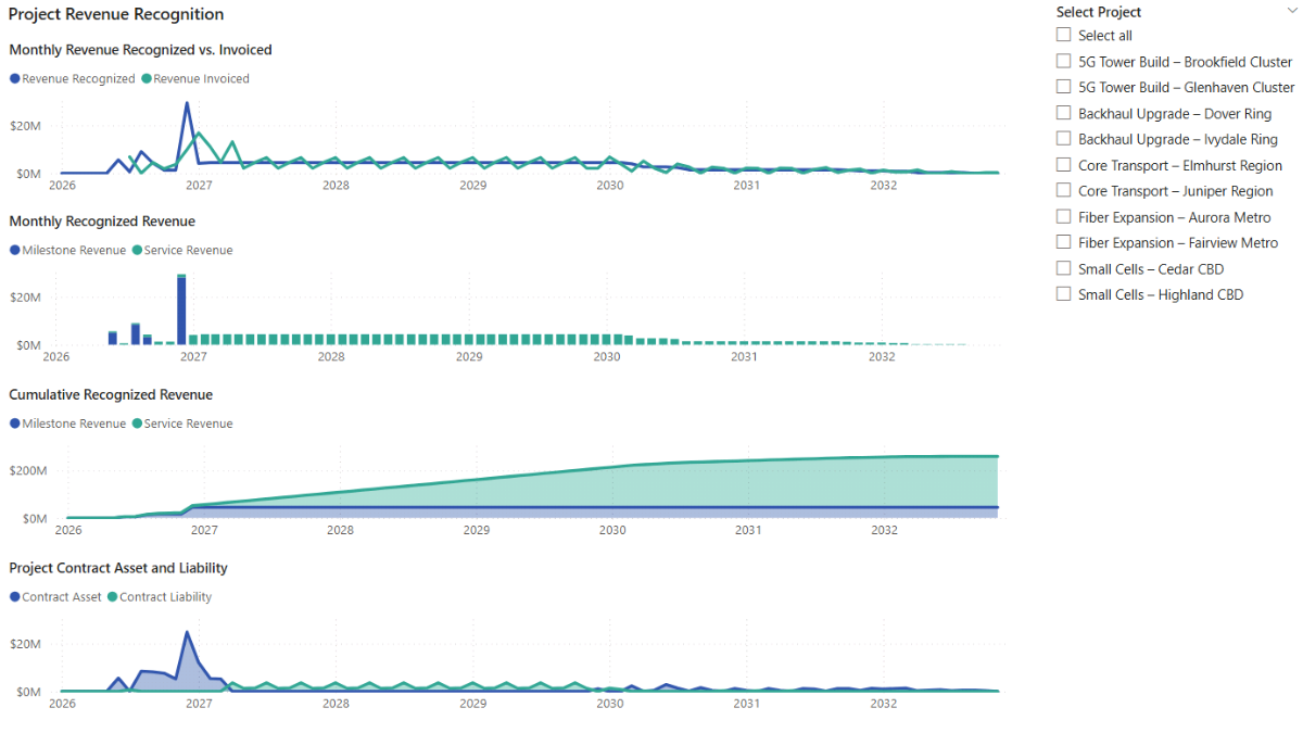
d. Project Contract Asset and Liability

This chart visualises how timing differences between revenue recognition and billing translate into contract assets and contract liabilities over time.

Insert an Area chart, add Calendar[MonthStart] to the X-axis, and add the Project Contract Asset and Project Contract Liability measures to the Y-axis. This visual complements the “Monthly Revenue Recognized vs. Invoiced” chart by showing the balance-sheet impact of those timing differences.

e. Project Selector

Finally, add a slicer to analyse revenue recognition profiles at the individual project level.

Insert a Slicer and add dim_projects[ProjectName] as the field. In the Format pane, choose the Vertical list option.

Step 6. Project Finance and Debt Forecast Modelling

Before we move into cash flow and returns, we introduce the project finance logic (external link) used throughout the model. In this step, Microsoft Power BI becomes a lightweight project finance model: CAPEX drives debt drawdowns, contract timelines anchor repayment, and What-If parameters let you stress-test assumptions without rewriting DAX.

The objective here is not to replicate a bank-grade loan model, but to create a transparent, time-aware debt forecast that reacts correctly to project progress and user-defined assumptions.

6.1 Create Project Financing What-If Parameters

We start by creating a small set of What-If parameters that represent the main sources of uncertainty in a project finance structure. These parameters will later appear as sliders on the Project Financing dashboard and allow you to test alternative leverage, interest, and repayment assumptions interactively.

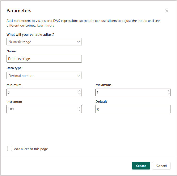
In Microsoft Power BI, go to Modeling → New parameter → Numeric range, and create the following parameters (the suggested ranges are typical for project financing, but adjust them to your use case):

Debt Leverage (Decimal number, min: 0, max: 1.0, increment: 0.01, default: 0)

Interest Rate (Decimal number, min: 0, max: 1.0, increment: 0.01, default: 0)

Debt Tenor Months (Whole number, min: 0, max: 120, increment: 6, default: 0)

Repayment Delay (Whole number, min: 0, max: 60, increment: 1, default: 0)

Opex % Revenue (Decimal number, min: 0, max: 1.0, increment: 0.01, default: 0)

Discount Rate (Decimal number, min: 0, max: 1.0, increment: 0.01, default: 0)

Clear the Add slicer to this page checkbox, as we’ll add the parameter slicers to the report later.

Each parameter automatically creates a supporting table and a default measure. In the next section, we define explicit assumption measures that reference these values and keep the financing DAX easier to read.

6.2 Project Financing Assumption Measures

After creating the What-If parameters, define a separate set of measures that reference the selected parameter values directly. Place these measures in a dedicated Parameters display folder so they are easy to find and reuse.

These measures act as stable inputs to the project finance model. Referencing them instead of the auto-generated parameter measures keeps the DAX easier to read and allows assumptions to be overridden later without changing slicers or parameter definitions.

p_LeveragePct

Returns the selected debt leverage percentage. Used throughout the debt draw, repayment, and outstanding balance calculations.

p_LeveragePct = 
    'Debt Leverage'[Debt Leverage Value]

p_InterestRate

Returns the selected annual interest rate. Drives the monthly interest expense calculation.

p_InterestRate = 
    'Interest Rate'[Interest Rate Value]

p_RepayTenorMonths

Returns the selected repayment tenor in months. Defines the length of the debt amortisation schedule.

p_RepayTenorMonths = 
    'Debt Tenor Months'[Debt Tenor Months Value]

p_RepayDelayMonths

Returns the repayment delay in months. Shifts the start of repayments relative to Ready for Service (RFS).

p_RepayDelayMonths = 
    'Repayment Delay'[Repayment Delay Value]

p_OpexPct

Returns the operating cost assumption as a percentage of service revenue. Used later in EBITDA and cash-flow calculations.

p_OpexPct = 
    'Opex % Revenue'[Opex % Revenue Value]

p_DiscountRate

Returns the selected discount rate. Used in project NPV calculations.

p_DiscountRate = 
    'Discount Rate'[Discount Rate Value]

These assumption measures are reused throughout the remaining project financing, cash-flow, and valuation calculations so that all results respond consistently to changes in leverage, interest rate, repayment timing, operating cost assumptions, and discount rate.

6.3 Project Finance Debt and Interest DAX Calculations

Before diving into the DAX, it’s worth clarifying the financing mechanics implemented in this model. At a high level, debt is drawn in proportion to monthly CAPEX, then repaid evenly after the project reaches Ready for Service (RFS) over the selected repayment tenor. Interest expense is calculated on the prior-period outstanding debt balance.

The measures below translate CAPEX forecasts and financing assumptions into a time-based debt forecast, covering debt capacity, drawdowns, repayments, outstanding balance, and interest expense.

Project Financing Eligible Debt

Defines the project’s debt capacity as a percentage of cumulative forecast CAPEX. Scales automatically with the size and timing of the investment.

Project Financing Eligible Debt = 
[Project CAPEX Cumulative Forecast] * [p_LeveragePct]

Project Financing Debt Outstanding

Tracks the outstanding debt balance over time by accumulating debt drawdowns and subtracting repayments. Acts as the central balance used for interest expense and credit metrics.

Project Financing Debt Outstanding =
VAR AsOfMonth = MAX ( Calendar[MonthStart] )
RETURN
SUMX (
    FILTER ( ALL ( Calendar[MonthStart] ), Calendar[MonthStart] <= AsOfMonth ),
    VAR m = Calendar[MonthStart]
    RETURN
        CALCULATE (
            [Project Financing Draw (Period)] - [Project Financing Repayment (Period)],
            FILTER ( ALL ( 'Calendar' ), Calendar[MonthStart] = m )
        )
)

Project Financing Draw (Period)

Models monthly debt drawdowns by applying the leverage assumption to forecast CAPEX in each month. Reflects progressive funding as capital is deployed during construction.

Project Financing Draw (Period) = 
VAR Lev = [p_LeveragePct]
RETURN
SUMX (
    VALUES ( Calendar[MonthStart] ),
    VAR CurMonth = Calendar[MonthStart]
    RETURN
        Lev
            * CALCULATE (
                [Project CAPEX (Forecast)],
                FILTER ( ALL ( 'Calendar' ), Calendar[MonthStart] = CurMonth )
            )
)

Project Financing Repayment (Period)

Models the monthly debt repayment schedule. Repayments start after RFS (plus any repayment delay) and amortize debt evenly across the selected repayment tenor, based on the remaining repayment window for each draw.

Project Financing Repayment (Period) = 
VAR Lev   = [p_LeveragePct]
VAR Delay = [p_RepayDelayMonths]
VAR Tenor = [p_RepayTenorMonths]
RETURN
SUMX (
    VALUES ( Calendar[MonthStart] ),
    VAR PayMonth = Calendar[MonthStart]
    RETURN
        SUMX (
            VALUES ( dim_projects[ProjectID] ),
            VAR RFS = CALCULATE ( MAX ( dim_projects[RFSDate] ) )
            VAR RepayStart =
                IF ( NOT ISBLANK ( RFS ), EDATE ( RFS, Delay ) )
            VAR RepayStartMonth =
                IF ( NOT ISBLANK ( RepayStart ), DATE ( YEAR ( RepayStart ), MONTH ( RepayStart ), 1 ) )
            VAR RepayEndMonth =
                IF ( NOT ISBLANK ( RepayStartMonth ), EDATE ( RepayStartMonth, Tenor - 1 ) )

            RETURN
                IF (
                    ISBLANK ( RepayStartMonth )
                        || PayMonth < RepayStartMonth
                        || PayMonth > RepayEndMonth,
                    0,
                    // Sum repayments contributed by each draw month (capex month)
                    SUMX (
                        FILTER (
                            ALL ( Calendar[MonthStart] ),
                            Calendar[MonthStart] <= PayMonth
                                && Calendar[MonthStart] <= RepayEndMonth
                        ),
                        VAR DrawMonth = Calendar[MonthStart]
                        VAR AmortStartMonth =
                            MAX ( DrawMonth, RepayStartMonth )
                        VAR RemainingMonths =
                            DATEDIFF ( AmortStartMonth, RepayEndMonth, MONTH ) + 1
                        VAR DrawAmt =
                            Lev
                                * CALCULATE (
                                    [Project CAPEX (Forecast)],
                                    FILTER ( ALL ( 'Calendar' ), Calendar[MonthStart] = DrawMonth )
                                )
                        RETURN
                            IF (
                                DrawAmt > 0
                                    && PayMonth >= AmortStartMonth
                                    && PayMonth <= RepayEndMonth,
                                DIVIDE ( DrawAmt, RemainingMonths, 0 ),
                                0
                            )
                    )
                )
        )
)

Project Financing Interest Expense (Period)

Calculates monthly interest expense using the prior month’s outstanding debt balance and the selected annual interest rate. Automatically responds to leverage, repayment timing, and tenor assumptions.

Project Financing Interest Expense (Period) = 
VAR Rate = [p_InterestRate]
RETURN
SUMX (
    VALUES ( Calendar[MonthStart] ),
    VAR CurMonth  = Calendar[MonthStart]
    VAR PrevMonth = EDATE ( CurMonth, -1 )
    VAR DebtPrev =
        CALCULATE (
            [Project Financing Debt Outstanding],
            FILTER ( ALL ( 'Calendar' ), Calendar[MonthStart] = PrevMonth )
        )
    RETURN
        DebtPrev * Rate / 12
)

Project Net Debt Movement (Period)

Captures the net monthly change in debt by subtracting repayments from drawdowns. Useful for reconciliation and cash-flow analysis.

Project Net Debt Movement (Period) = 
[Project Financing Draw (Period)] - [Project Financing Repayment (Period)]

6.4 Project Financing Dashboard

In this section, we bring the project finance measures together into a dedicated Power BI dashboard. The goal is to make financing assumptions explicit, show how debt is drawn and repaid over time, and visualise the resulting debt balance and interest expense across the project lifecycle.

a. Financing Parameters

These slicers control the core assumptions of the project finance model: how much of CAPEX is financed with debt, the annual interest rate, the length of the repayment period, and any delay between project completion and the start of debt amortisation.

Go to Report view → Home → Visuals gallery and insert Slicer visuals, using the Debt Leverage, Interest Rate, Debt Tenor Months, and Repayment Delay parameters as the slicer fields. For each slicer, open the Format pane, select the Single value option, enable the Slider, and adjust the slicer header text so the assumptions are clearly labelled.

b. Monthly Project Financing (Draws and Repayments)

This chart shows how project financing is drawn during construction and repaid once the project becomes operational. It provides a clear view of the debt funding profile and the repayment schedule implied by the selected assumptions.

Insert a Stacked column chart, add Calendar[MonthStart] to the X-axis, and add the Project Financing Draw (Period) and Project Financing Repayment (Period) measures to the Y-axis. Right-click each measure and select Rename for this visual to adjust labels, then use the Format pane to remove axis titles and refine the legend and chart title.

c. Cumulative CAPEX and Debt Balance

This visual compares cumulative investment against outstanding debt over time. It highlights how leverage and repayment assumptions translate into the evolving debt balance across the project’s lifetime.

Insert a Stacked area chart, add Calendar[MonthStart] to the X-axis, and add Project CAPEX Cumulative Forecast and Project Financing Debt Outstanding to the Y-axis. Rename fields where needed and apply consistent formatting.

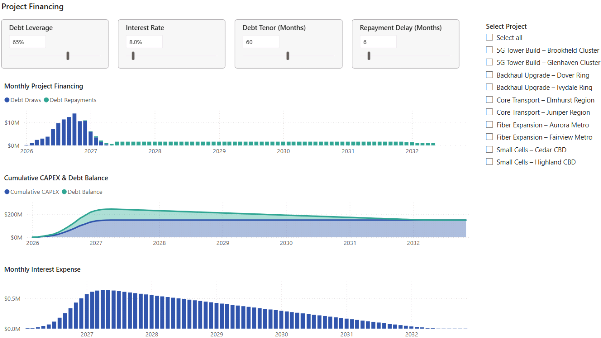
d. Monthly Interest Expense

This chart shows the monthly interest cost associated with project financing. Because interest is calculated on the outstanding debt balance, it responds directly to changes in leverage, repayment timing, tenor, and interest rate.

Insert a Clustered column chart, add Calendar[MonthStart] to the X-axis, and add Project Financing Interest Expense (Period) to the Y-axis. Use the Format pane to remove axis titles and adjust the chart title formatting.

e. Project Selector

Finally, add a slicer to analyse project financing profiles at the individual project level.

Insert a Slicer and add dim_projects[ProjectName] as the field. In the Format pane, select the Vertical list option.

Step 7. Cash Flow, Returns, and Project Finance Metrics

In this step we move from revenue recognition and debt forecasting into the investment view of the project: cash flow, profitability, and returns. The measures here connect billing, operating costs, CAPEX, and project financing into a single timeline so you can see when projects consume cash, when they start generating cash, and how leverage changes the risk/return profile.

This step also sets up the Cash Flow and Returns dashboard page. Because these calculations are reused across visuals, slicers, and scenario parameters, the DAX measures are written to stay stable under different Calendar views while still responding correctly when you switch projects or adjust assumptions.

7.1 OPEX and Earnings Measures (EBITDA)

Project OPEX (Period)

Estimates operating expenses as a percentage of recognized service revenue. This simplification reflects the fact that ongoing operating costs typically scale with recurring service activity rather than milestone events.

Project OPEX (Period) = 
[Project Revenue Recognized (Service, Period)] * [p_OpexPct]

Project EBITDA (Period)

Calculates EBITDA as recognized revenue minus operating expenses. Acts as the core earnings measure used later in leverage ratios and debt service coverage calculations.

Project EBITDA (Period) :=
[Project Revenue Recognized (Period)] - [Project OPEX (Period)]

Project EBITDA (TTM)

Calculates trailing twelve-month (TTM) EBITDA to smooth short-term volatility and provide a rolling view of earnings capacity.

Project EBITDA (TTM) :=
CALCULATE (
    [Project EBITDA (Period)],
    DATESINPERIOD ( Calendar[Date], MAX ( Calendar[Date] ), -12, MONTH )
)

Project EBITDA Margin

Expresses EBITDA as a percentage of recognized revenue, enabling profitability comparisons across projects of different sizes.

Project EBITDA Margin :=
VAR Rev = [Project Revenue Recognized (Period)]
RETURN
IF ( Rev > 0, DIVIDE ( [Project EBITDA (Period)], Rev ) )

7.2 Unlevered and Levered Cash Flow Measures

Creates two cash-flow views: unlevered (pre-debt) and levered (post-financing). This split is central to project finance analysis. Unlevered cash flow tests whether the project works economically on its own, while levered cash flow reflects the equity investor’s experience after debt drawdowns, repayments, and interest.

Project Net Cash Flow (Unlevered, Period)

Calculates unlevered cash flow as billing minus operating expenses and CAPEX in each period. Uses billing rather than recognized revenue to better approximate cash collection timing.

Project Net Cash Flow (Unlevered, Period) =
[Project Billing (Period)]
- [Project OPEX (Period)]
- [Project CAPEX (Forecast)]

Project Net Cash Flow (Levered, Period)

Converts unlevered cash flow into levered cash flow by incorporating project financing. Adds debt drawdowns and subtracts repayments and interest expense.

Project Net Cash Flow (Levered, Period) :=
[Project Net Cash Flow (Unlevered, Period)]
+ [Project Financing Draw (Period)]
- [Project Financing Repayment (Period)]
- [Project Financing Interest Expense (Period)]

Project Net Cash Flow (Unlevered, Cumulative)

Accumulates unlevered cash flow over time to approximate the project’s cash balance and support payback analysis.

Project Net Cash Flow (Unlevered, Cumulative) :=
VAR AsOfMonth = MAX ( Calendar[MonthStart] )
RETURN
SUMX (
    FILTER ( ALL ( Calendar[MonthStart] ), Calendar[MonthStart] <= AsOfMonth ),
    CALCULATE ( [Project Net Cash Flow (Unlevered, Period)] )
)

Project Net Cash Flow (Levered, Cumulative)

Accumulates levered cash flow over time to represent the equity-level cash balance. Reflects the combined impact of operating performance and financing structure.

Project Net Cash Flow (Levered, Cumulative) :=
VAR AsOfMonth = MAX ( Calendar[MonthStart] )
RETURN
SUMX (
    FILTER ( ALL ( Calendar[MonthStart] ), Calendar[MonthStart] <= AsOfMonth ),
    CALCULATE ( [Project Net Cash Flow (Levered, Period)] )
)

7.3 Project NPV and IRR Calculations (Unlevered and Levered)

Assumes the project is fully closed out at the end of the contract. Any remaining financial position—outstanding debt, contract assets, or contract liabilities—is settled in the final month and reflected as a terminal cash-flow adjustment.

Project Terminal Adjustment (Levered)

Applies a one-time close-out adjustment in the final contract month. Adds contract assets, subtracts contract liabilities, and subtracts any remaining outstanding debt to approximate the cash impact of settling the project at termination.

Project Terminal Adjustment (Levered) :=
VAR StartMonth =
    CALCULATE ( MIN ( fct_capex[MonthStart] ), REMOVEFILTERS ( Calendar ) )
VAR EndMonthRaw =
    CALCULATE ( MAX ( dim_contracts[ContractEnd] ), REMOVEFILTERS ( Calendar ) )
VAR EndMonth =
    IF ( NOT ISBLANK ( EndMonthRaw ), DATE ( YEAR ( EndMonthRaw ), MONTH ( EndMonthRaw ), 1 ) )
VAR CurMonth = MAX ( Calendar[MonthStart] )
RETURN
IF (
    ISBLANK ( StartMonth ) || ISBLANK ( EndMonth ) || CurMonth <> EndMonth,
    0,
    + [Project Contract Asset]
    - [Project Contract Liability]
    - [Project Financing Debt Outstanding]
)

Project Net Cash Flow (Levered, Period, Terminal)

Extends the levered cash-flow series by adding the terminal adjustment in the final month, producing a complete equity cash-flow stream for valuation.

Project Net Cash Flow (Levered, Period, Terminal) :=
[Project Net Cash Flow (Levered, Period)]
+ [Project Terminal Adjustment (Levered)]

NPV and IRR are calculated over a fixed project window that is independent of the Calendar axis used in visuals. This prevents valuation metrics from changing when you zoom charts or switch time granularities. Results respond only to project selection and assumption changes.

Project NPV (Unlevered)

Discounts the monthly unlevered cash-flow stream from the first CAPEX month to the final contract month using a monthly discount rate derived from the selected annual discount rate.

Project NPV (Unlevered) :=
VAR r_annual =
    [p_DiscountRate]
VAR r_month =
    POWER ( 1 + r_annual, 1/12 ) - 1

VAR StartMonth =
    CALCULATE ( MIN ( fct_capex[MonthStart] ), REMOVEFILTERS ( Calendar ) )
VAR EndMonthRaw =
    CALCULATE ( MAX ( dim_contracts[ContractEnd] ), REMOVEFILTERS ( Calendar ) )
VAR EndMonth =
    DATE ( YEAR ( EndMonthRaw ), MONTH ( EndMonthRaw ), 1 )

VAR NMonths =
    DATEDIFF ( StartMonth, EndMonth, MONTH )

RETURN
IF (
    ISBLANK ( StartMonth ) || ISBLANK ( EndMonthRaw ) || NMonths < 0,
    BLANK (),
    SUMX (
        GENERATESERIES ( 0, NMonths, 1 ),
        VAR k = [Value]
        VAR m = EDATE ( StartMonth, k )
        VAR cf =
            CALCULATE (
                [Project Net Cash Flow (Unlevered, Period)],
                FILTER ( ALL ( Calendar[MonthStart] ), Calendar[MonthStart] = m )
            )
        RETURN
            DIVIDE ( cf, POWER ( 1 + r_month, k ), 0 )
    )
)

Project NPV (Levered)

Discounts the monthly levered cash-flow stream, including the terminal adjustment, to produce an equity-level NPV.

Project NPV (Levered) :=
VAR r_annual =
    [p_DiscountRate]
VAR r_month =
    POWER ( 1 + r_annual, 1/12 ) - 1

VAR StartMonth =
    CALCULATE ( MIN ( fct_capex[MonthStart] ), REMOVEFILTERS ( 'Calendar' ) )
VAR EndMonthRaw =
    CALCULATE ( MAX ( dim_contracts[ContractEnd] ), REMOVEFILTERS ( 'Calendar' ) )
VAR EndMonth =
    IF ( NOT ISBLANK ( EndMonthRaw ), DATE ( YEAR ( EndMonthRaw ), MONTH ( EndMonthRaw ), 1 ) )

VAR NMonths =
    DATEDIFF ( StartMonth, EndMonth, MONTH )

RETURN
IF (
    ISBLANK ( StartMonth ) || ISBLANK ( EndMonth ) || NMonths < 0,
    BLANK (),
    SUMX (
        GENERATESERIES ( 0, NMonths, 1 ),
        VAR k = [Value]
        VAR m = EDATE ( StartMonth, k )
        VAR cf =
            CALCULATE (
                [Project Net Cash Flow (Levered, Period, Terminal)],
                FILTER ( ALL ( 'Calendar' ), Calendar[MonthStart] = m )
            )
        RETURN
            DIVIDE ( cf, POWER ( 1 + r_month, k ), 0 )
    )
)

Project IRR (Unlevered)

Calculates the internal rate of return on the unlevered cash-flow stream using XIRR. Includes validation checks to ensure the cash-flow series contains both negative and positive values.

Project IRR (Unlevered) = 
VAR StartMonth =
    CALCULATE ( MIN ( fct_capex[MonthStart] ), REMOVEFILTERS ( 'Calendar' ) )
VAR EndMonthRaw =
    CALCULATE ( MAX ( dim_contracts[ContractEnd] ), REMOVEFILTERS ( 'Calendar' ) )
VAR EndMonth =
    IF ( NOT ISBLANK ( EndMonthRaw ), DATE ( YEAR ( EndMonthRaw ), MONTH ( EndMonthRaw ), 1 ) )
VAR NMonths =
    DATEDIFF ( StartMonth, EndMonth, MONTH )

VAR t =
    ADDCOLUMNS (
        GENERATESERIES ( 0, NMonths, 1 ),
        "Dt", EDATE ( StartMonth, [Value] ),
        "CF",
            CALCULATE (
                [Project Net Cash Flow (Unlevered, Period)],
                FILTER ( ALL ( 'Calendar' ), Calendar[MonthStart] = EDATE ( StartMonth, [Value] ) )
            )
    )

VAR HasNeg = MINX ( t, [CF] ) < 0
VAR HasPos = MAXX ( t, [CF] ) > 0
VAR SumAbs = SUMX ( t, ABS ( [CF] ) )

VAR IRR_Value =
    IFERROR ( XIRR ( t, [CF], [Dt], 0.10 ), BLANK () )

RETURN
IF (
    ISBLANK ( StartMonth ) || ISBLANK ( EndMonth ) || NMonths < 0 || SumAbs = 0 || NOT ( HasNeg && HasPos ),
    BLANK (),
    IRR_Value
)

Project IRR (Levered)

Calculates equity IRR on the levered cash-flow stream using XIRR. Typically more sensitive to interest rate, leverage, and repayment assumptions than unlevered IRR.

Project IRR (Levered) :=
VAR StartMonth =
    CALCULATE ( MIN ( fct_capex[MonthStart] ), REMOVEFILTERS ( 'Calendar' ) )
VAR EndMonthRaw =
    CALCULATE ( MAX ( dim_contracts[ContractEnd] ), REMOVEFILTERS ( 'Calendar' ) )
VAR EndMonth =
    IF ( NOT ISBLANK ( EndMonthRaw ), DATE ( YEAR ( EndMonthRaw ), MONTH ( EndMonthRaw ), 1 ) )
VAR NMonths =
    DATEDIFF ( StartMonth, EndMonth, MONTH )

VAR t =
    ADDCOLUMNS (
        GENERATESERIES ( 0, NMonths, 1 ),
        "Dt", EDATE ( StartMonth, [Value] ),
        "CF",
            CALCULATE (
                [Project Net Cash Flow (Levered, Period, Terminal)],
                FILTER ( ALL ( 'Calendar' ), Calendar[MonthStart] = EDATE ( StartMonth, [Value] ) )
            )
    )

VAR HasNeg = MINX ( t, [CF] ) < 0
VAR HasPos = MAXX ( t, [CF] ) > 0
VAR SumAbs = SUMX ( t, ABS ( [CF] ) )

VAR IRR_Value =
    IFERROR ( XIRR ( t, [CF], [Dt], 0.15 ), BLANK () )

RETURN
IF (
    ISBLANK ( StartMonth ) || ISBLANK ( EndMonth ) || NMonths < 0 || SumAbs = 0 || NOT ( HasNeg && HasPos ),
    BLANK (),
    IRR_Value
)

7.4 Project Payback Calculations

Uses payback as a simple, cash-based liquidity metric. Measures how long it takes for cumulative cash flow to return to zero (or above). In project finance analysis, payback complements NPV and IRR as a quick indicator of capital recovery and risk.

Project Payback Month (Unlevered)

Identifies the first month in which cumulative unlevered cash flow becomes non-negative.

Project Payback Month (Unlevered) :=
VAR StartMonth =
    CALCULATE ( MIN ( fct_capex[MonthStart] ), REMOVEFILTERS ( 'Calendar' ) )
VAR EndMonthRaw =
    CALCULATE ( MAX ( dim_contracts[ContractEnd] ), REMOVEFILTERS ( 'Calendar' ) )
VAR EndMonth =
    DATE ( YEAR ( EndMonthRaw ), MONTH ( EndMonthRaw ), 1 )
VAR NMonths =
    DATEDIFF ( StartMonth, EndMonth, MONTH )

VAR t =
    ADDCOLUMNS (
        GENERATESERIES ( 0, NMonths, 1 ),
        "Dt", EDATE ( StartMonth, [Value] ),
        "CF",
            CALCULATE (
                [Project Net Cash Flow (Unlevered, Period)],
                FILTER ( ALL ( Calendar[MonthStart] ), Calendar[MonthStart] = EDATE ( StartMonth, [Value] ) )
            )
    )

VAR tCum =
    ADDCOLUMNS (
        t,
        "CumCF",
            VAR k = [Value]
            RETURN SUMX ( FILTER ( t, [Value] <= k ), [CF] )
    )

RETURN
IF (
    ISBLANK ( StartMonth ) || ISBLANK ( EndMonthRaw ) || NMonths < 0,
    BLANK (),
    MINX ( FILTER ( tCum, [CumCF] >= 0 ), [Dt] )
)

Project Payback Month (Levered)

Identifies the payback month for the levered cash-flow series, reflecting the equity investor’s capital recovery timeline after financing flows.

Project Payback Month (Levered) =
VAR StartMonth =
    CALCULATE ( MIN ( fct_capex[MonthStart] ), REMOVEFILTERS ( 'Calendar' ) )
VAR EndMonthRaw =
    CALCULATE ( MAX ( dim_contracts[ContractEnd] ), REMOVEFILTERS ( 'Calendar' ) )
VAR EndMonth =
    IF ( NOT ISBLANK ( EndMonthRaw ), DATE ( YEAR ( EndMonthRaw ), MONTH ( EndMonthRaw ), 1 ) )
VAR NMonths =
    DATEDIFF ( StartMonth, EndMonth, MONTH )

VAR t =
    ADDCOLUMNS (
        GENERATESERIES ( 0, NMonths, 1 ),
        "Dt", EDATE ( StartMonth, [Value] ),
        "CF",
            CALCULATE (
                [Project Net Cash Flow (Levered, Period, Terminal)],
                FILTER ( ALL ( 'Calendar' ), Calendar[MonthStart] = EDATE ( StartMonth, [Value] ) )
            )
    )

VAR tCum =
    ADDCOLUMNS (
        t,
        "CumCF",
            VAR k = [Value]
            RETURN SUMX ( FILTER ( t, [Value] <= k ), [CF] )
    )
RETURN
IF (
    ISBLANK ( StartMonth ) || ISBLANK ( EndMonth ) || NMonths < 0,
    BLANK (),
    MINX ( FILTER ( tCum, [CumCF] >= 0 ), [Dt] )
)

Project Payback (Months, Unlevered)

Converts the unlevered payback date into a number of months from the first CAPEX month.

Project Payback (Months, Unlevered) :=
VAR StartMonth =
    CALCULATE ( MIN ( fct_capex[MonthStart] ), REMOVEFILTERS ( 'Calendar' ) )
VAR PB = [Project Payback Month (Unlevered)]
RETURN
IF ( NOT ISBLANK ( StartMonth ) && NOT ISBLANK ( PB ), DATEDIFF ( StartMonth, PB, MONTH ) )

Project Payback (Months, Levered)

Converts the levered payback date into a number of months from the first CAPEX month.

Project Payback (Months, Levered) :=
VAR StartMonth =
    CALCULATE ( MIN ( fct_capex[MonthStart] ), REMOVEFILTERS ( 'Calendar' ) )
VAR PB = [Project Payback Month (Levered)]
RETURN
IF ( NOT ISBLANK ( StartMonth ) && NOT ISBLANK ( PB ), DATEDIFF ( StartMonth, PB, MONTH ) )

7.5 Cash Flow and Returns Dashboard

With cash flow and valuation measures in place, we can now build a dashboard page that summarises investment performance and visualises cash movements over time for both unlevered and levered scenarios.

a. Key financial metrics (cards)

Go to Report view → Home → Visuals gallery and insert a Card (new) visual. Add the Project NPV (Levered), Project NPV (Unlevered), Project IRR (Levered), Project IRR (Unlevered), Project Payback (Months, Levered), and Project Payback (Months, Unlevered) measures to the card. Right-click each field and select Rename for this visual to adjust labels, then use the Format pane (Layout, Callout values, Cards) to style the headline metrics.

b. Slicers

Insert three slicers: add dim_projects[ProjectName] as a dropdown slicer, then add the Opex % Revenue and Discount Rate parameters as slider slicers so the cash flow and valuation results respond to assumption changes.

c. Monthly project cash flow movements

Insert a Clustered column chart, add Calendar[MonthStart] to the X-axis, and add the Project Net Cash Flow (Unlevered, Period) and Project Net Cash Flow (Levered, Period) measures to the Y-axis. Rename measures for readability and remove axis titles to keep the chart clean.

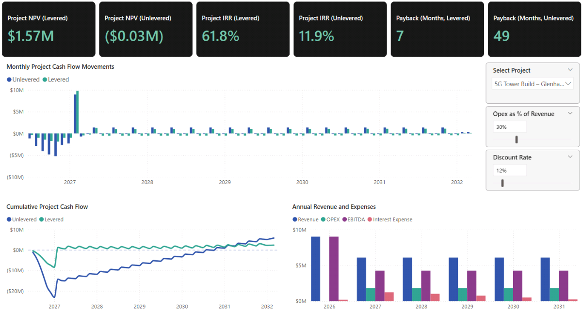
d. Cumulative cash flow balance

Insert a Line chart, add Calendar[MonthStart] to the X-axis, and add the Project Net Cash Flow (Unlevered, Cumulative) and Project Net Cash Flow (Levered, Cumulative) measures to the Y-axis. Add a constant line at 0 on the Y-axis (Analytics / Reference lines) so the payback points are visually obvious.

e. Annual revenue and expenses

Insert a Clustered column chart, add Calendar[Year] to the X-axis, and add Project Revenue Recognized (Period), Project OPEX (Period), Project EBITDA (Period), and Project Financing Interest Expense (Period) to the Y-axis. This gives a compact annual view of operational performance and financing costs.

7.6 Making Dashboard Timelines Dynamic

To dynamically adjust a visual’s timeline to the selected project window, go to the Filter pane and add the Show Period (In Project Window) measure (DAX code below) to the Filters on this visual section. Then set the filter to show items when the value equals 1.

Project Window Start Month

This measure returns the earliest CAPEX month in the current selection. REMOVEFILTERS ensures the start month is calculated across the full project window, not just within the visible portion of the Calendar.

Project Window Start Month :=
CALCULATE ( MIN ( fct_capex[MonthStart] ), REMOVEFILTERS ( Calendar ) )

Project Window End Month

This measure returns the final contract month in the current selection, which acts as the end of the project window for reporting purposes.

Project Window End Month :=
VAR EndRaw =
    CALCULATE ( MAX ( dim_contracts[ContractEnd] ), REMOVEFILTERS ( Calendar ) )
RETURN
IF ( NOT ISBLANK ( EndRaw ), DATE ( YEAR ( EndRaw ), MONTH ( EndRaw ), 1 ) )

Show Period (In Project Window)

This measure returns 1 when the current month falls within the project window and 0 otherwise. It uses as a visual-level filter to automatically hide months outside the active project timeline.

Show Period (In Project Window) :=
VAR m = MAX ( Calendar[MonthStart] )
VAR StartM = [Project Window Start Month]
VAR EndM   = [Project Window End Month]
RETURN
IF ( NOT ISBLANK ( StartM ) && NOT ISBLANK ( EndM ) && m >= StartM && m <= EndM, 1, 0 )

7.7 Syncing Parameters and Power BI Dashboards

To make sure the Project Finance parameters and other assumption slicers apply consistently across pages, use Microsoft Power BI’s Sync slicers feature.

Go to the page where the parameter slicers are configured (for example, Project Financing). Click a parameter slicer (for example, Debt Leverage), then click on the Sync slicers icon on the right sidebar. In the Sync slicers pane, tick the pages where you want that same parameter to apply (for example, Cash Flow and Financial Summary), and choose whether it should be visible on those pages or synced in the background. Repeat the same steps for the remaining parameter slicers.

Step 8. Debt Service, Credit Metrics, and Scenario Analysis

In this final step, we shift from building the project finance model to interpreting it like a lender or investment committee would. We translate the debt forecast and cash-flow outputs into credit-style metrics (leverage, coverage, and DSCR), then consolidate the model into a Financials Summary page for decision-making.

To finish, we run a small set of structured scenarios. This is the point of a Power BI dashboard. It is not about testing random slider combinations, but about defining a few realistic cases and seeing how assumptions compound through cash flow and returns.

8.1 Debt, Equity, and Credit Metrics DAX Measures

Converts project financing outputs into standard credit metrics used in project finance. All measures respond dynamically to project selection and key assumptions (leverage, interest rate, tenor, OPEX %, discount rate), allowing the debt profile to be evaluated under different scenarios.

Project Equity Invested (Cumulative)

Estimates cumulative equity invested as the portion of cumulative CAPEX not funded by debt. Acts as a simple proxy for equity contribution over time.

Project Equity Invested (Cumulative) :=
[Project CAPEX Cumulative Forecast] - [Project Financing Debt Outstanding]

Project Equity Invested (Cumulative, Non-Negative)

Floors cumulative equity invested at zero to avoid negative equity values when debt timing temporarily exceeds CAPEX in edge cases.

Project Equity Invested (Cumulative, Non-Negative) :=
MAX ( 0, [Project Equity Invested (Cumulative)] )

Project Debt to Equity

Expresses leverage as outstanding debt divided by cumulative equity invested.

Project Debt to Equity :=
VAR Eq = [Project Equity Invested (Cumulative, Non-Negative)]
RETURN
IF ( Eq > 0, DIVIDE ( [Project Financing Debt Outstanding], Eq ) )

Project Debt to EBITDA

Compares outstanding debt to trailing twelve-month EBITDA, a standard debt multiple used in credit analysis.

Project Debt to EBITDA :=
VAR Den = [Project EBITDA (TTM)]
RETURN
IF ( Den > 0, DIVIDE ( [Project Financing Debt Outstanding], Den ) )

Project Interest Coverage

Measures how comfortably trailing twelve-month EBITDA covers trailing twelve-month interest expense.

Project Interest Coverage :=
VAR Den =
    CALCULATE (
        [Project Financing Interest Expense (Period)],
        DATESINPERIOD ( Calendar[Date], MAX ( Calendar[Date] ), -12, MONTH )
    )
VAR Num = [Project EBITDA (TTM)]
RETURN
IF ( Den > 0, DIVIDE ( Num, Den ) )

Project Debt Service (Period)

Defines total debt service as scheduled principal repayment plus interest expense in the period.

Project Debt Service (Period) :=
[Project Financing Interest Expense (Period)] + [Project Financing Repayment (Period)]

DSCR (EBITDA, TTM)

Calculates a DSCR-style ratio using trailing twelve-month EBITDA as the numerator and trailing twelve-month debt service as the denominator.

DSCR (EBITDA, TTM) :=
VAR Num =
    CALCULATE (
        [Project EBITDA (Period)],
        DATESINPERIOD ( Calendar[Date], MAX ( Calendar[Date] ), -12, MONTH )
    )
VAR Den =
    CALCULATE (
        [Project Debt Service (Period)],
        DATESINPERIOD ( Calendar[Date], MAX ( Calendar[Date] ), -12, MONTH )
    )
RETURN
IF ( Den > 0, DIVIDE ( Num, Den ) )

DSCR (Cash, TTM)

Calculates a cash-based DSCR using unlevered cash flow as the numerator. Better approximates cash available for debt service in project finance analysis.

DSCR (Cash, TTM) :=
VAR Num =
    CALCULATE (
        [Project Net Cash Flow (Unlevered, Period)],
        DATESINPERIOD ( Calendar[Date], MAX ( Calendar[Date] ), -12, MONTH )
    )
VAR Den =
    CALCULATE (
        [Project Debt Service (Period)],
        DATESINPERIOD ( Calendar[Date], MAX ( Calendar[Date] ), -12, MONTH )
    )
RETURN
IF ( Den > 0, DIVIDE ( Num, Den ) )

Project Applied Leverage (Cumulative)

Checks applied leverage by comparing cumulative debt drawn to cumulative CAPEX. Useful for validating that debt draw behaviour matches the intended leverage assumption.

Project Applied Leverage (Cumulative) :=
VAR AsOfMonth = MAX ( Calendar[MonthStart] )
VAR CapexCum  = [Project CAPEX Cumulative Forecast]
VAR DebtCum =
    SUMX (
        FILTER ( ALL ( Calendar[MonthStart] ), Calendar[MonthStart] <= AsOfMonth ),
        CALCULATE ( [Project Financing Draw (Period)] )
    )
RETURN
DIVIDE ( DebtCum, CapexCum )

Project Cash Balance (Levered)

Uses cumulative levered cash flow as a proxy for project-level cash balance under the selected financing structure.

Project Cash Balance (Levered) :=
[Project Net Cash Flow (Levered, Cumulative)]

8.2 Financials Summary Dashboard

This dashboard is designed as a decision page, which consolidates annual performance, cash flow, and credit metrics into two matrices so you can review a project like a mini investment memo.

a. Project Name selector

Go to Report view → Home → Visuals gallery and insert a Slicer. Add dim_projects[ProjectName] as the field, then go to the Slicer settings in the Format pane and choose the Dropdown option.

b. Annual Project Cash Flow and Revenue

This matrix summarises key annual financials including billed and recognized revenue, earnings, CAPEX, and both unlevered and levered cash flows.

Insert a Matrix, add Calendar[Year] (or Year/Quarter for more granularity) to Rows, and add Project Billing (Period), Project Revenue Recognized (Period), Project OPEX (Period), Project EBITDA (Period), Project CAPEX (Forecast), Project Net Cash Flow (Unlevered, Period), Project Net Debt Movement (Period), Project Financing Interest Expense (Period), and Project Net Cash Flow (Levered, Period) to Columns. Right-click any field and select Rename for this visual where needed, then adjust column header formatting in the Format pane.

c. Debt Service and Credit Metrics

This matrix consolidates the core credit metrics used to assess leverage and debt-servicing capacity.

Insert a second Matrix, add Calendar[Year] to Rows, and add Project EBITDA (Period), Project Net Cash Flow (Unlevered, Period), Project Financing Interest Expense (Period), Project Financing Debt Outstanding, Project Equity Invested (Cumulative, Non-Negative), Project Debt to Equity, Project Debt to EBITDA, Project Debt Service (Period), DSCR (Cash, TTM), DSCR (EBITDA, TTM), and Project Interest Coverage to Columns. Rename fields for readability and format column headers consistently with the first matrix.

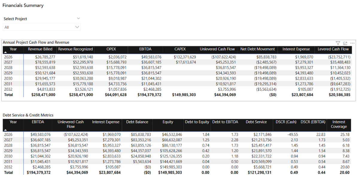
Remember to sync slicers and parameters from the Project Financing and Cash Flow pages so changes in leverage, interest rate, tenor, OPEX %, and discount rate carry through into this Financials Summary page.

8.3 What-If Scenarios and Sensitivity Analysis

With the dashboard built, the final step is interpretation. Rather than testing arbitrary combinations of sliders, define a small number of realistic scenarios and observe how risk compounds across cost, timeline, financing, and cash flow.

Scenario 1 — Base case (unlevered benchmark)

Base: 5G Tower Building – Glenhaven Cluster. $25m CAPEX, $41m total contract value. With OPEX set to 30% of service revenue (which equals $32m of the total contract value) and a 12% discount rate as the minimum return benchmark, the NPV is around break-even. Increasing OPEX to 35% pushes NPV to -$1.2m, which makes the base case unattractive on an unlevered basis.

Scenario 2 — Levered case (project financing improves equity profile)

Levered: 65% leverage and 8.0% interest rate. Even with 35% OPEX, NPV remains slightly positive at ca. $0.42m with an IRR of 31.2%. With OPEX back at 30%, NPV improves to  ca. $1.6m, showing how project financing can improve the equity cash-flow profile when the cost of debt is reasonable.

Scenario 3 — Higher interest rate (weak spot test)

Higher interest: increasing the interest rate from 8% to 12% pushes NPV back toward break-even and reduces IRR to ca. 11.5%, which falls below the 12% discount rate threshold. In this model, that sensitivity makes interest rate a key weak spot: higher debt costs can erase the benefit of leverage and make the project finance structure less attractive than the base case.

📌 Recap: Building a Project Financing & Revenue Recognition Dashboard in Microsoft Power BI

Here’s a quick recap of the steps required to build a complete project financing and revenue recognition dashboard in Microsoft Power BI:

1. Load and review project finance data. Import the projects, contracts, CAPEX, and billing tables, then validate key date and numeric fields so the model is reliable for time-based financial analysis.
2. Build the Calendar table and data model. Create a DAX Calendar table, mark it as a date table, and define clean one-to-many relationships so time filters flow correctly across CAPEX, billing, projects, and contracts.
3. Create core DAX measures for CAPEX and contract values. Define base measures for forecast CAPEX, cumulative CAPEX, budgets, contract transaction price, and milestone vs service allocations.
4. Build the core report pages. Create Projects Overview and Projects Detail pages to validate CAPEX, billing, and contract value behaviour before layering in accounting and financing logic.
5. Implement revenue recognition (milestone and service). Build DAX measures for milestone recognition at RFS, straight-line service revenue over the contract term, and contract assets/liabilities driven by timing differences vs billing.
6. Model project financing and debt forecasting. Add What-If parameters for leverage, interest, tenor, and repayment delay, then build debt draw, repayment, debt balance, and interest expense measures.
7. Build cash flow and returns metrics. Create unlevered vs levered cash flow, EBITDA, cumulative cash balance, and valuation measures (NPV, IRR, payback) with a consistent project window.
8. Add credit metrics and scenario analysis. Calculate debt service and lender-style ratios (leverage, coverage, DSCR), then consolidate results into a Financials Summary page for decision-making and scenario testing.

By following these steps, you now have a flexible Power BI model that connects CAPEX, contracts, billing, revenue recognition, and project financing into a single time-aware dashboard for analysis and scenario testing.

🔎 Preview the Interactive Project Financing and Revenue Recognition Dashboard

Explore the finished Project Financing & Revenue Recognition dashboard — the same model built in this tutorial. Adjust leverage, interest rate, repayment timing, OPEX %, and discount rate assumptions, and immediately see the impact on debt, revenue recognition, cash flow, returns, and credit metrics.

📥 Download My Project Financing & Revenue Recognition Dashboard Template

To help you get started quickly, I’ve prepared a ready-to-use Power BI template that includes:

• A complete Power BI (.pbix) file with revenue recognition, contract assets/liabilities, debt forecasting, cash flow, returns, and credit metrics already built.
• CSV input files for projects, contracts, CAPEX, billing, and calendar setup.
• A full DAX measure library, structured and grouped exactly as shown throughout this tutorial.

This template lets you adapt the model to your own projects, compare billing vs recognized revenue, forecast debt and interest, and run structured scenario testing without rebuilding everything from scratch.

👁️ View full template details

Get in Touch

Hi, I’m Jacek. I’m passionate about Microsoft Power BI, DAX, and analytical project and financial models.

I hope this tutorial helped you understand how to build a structured project finance and revenue recognition dashboard with debt forecasting, cash flow, and scenario analysis.

If you’d like support with project modelling, contract accounting logic, or Power BI dashboards, feel free to get in touch.

You can also explore more step-by-step tutorials, or check out my One-to-One Training and Data Analytics Support if you’d like personalised guidance.

Disclaimer: This tutorial is for informational and educational purposes only and should not be considered professional advice.

Explore More Tutorials

• • Power BI Project Planning & Cost Management Dashboard Tutorial — Build a structured project planning model that connects schedule, resources, costs, and cash flow.
  • Power BI Project Cost Allocation Dashboard Tutorial — Build a transparent project cost allocation model using allocation drivers, structured DAX, and interactive visuals.
  • Power BI Financial Planning & Analysis Dashboard Tutorial — Create a full FP&A model with forecasting, cash flow analysis, and scenario-driven financial planning.
  • Project Finance Model – Excel Tutorial — Learn how to structure a full project finance model in Microsoft Excel, including cash flow, debt, and return analysis.
  • Capital Investment Plan – Excel Tutorial — Build a capital investment plan in Excel to prioritise projects, phase CAPEX, and evaluate funding needs.