How to Build a Sales Analysis and Forecast Dashboard in Microsoft Power BI

Last Updated on January 4, 2026

In this tutorial, we’ll build a complete sales revenue analysis in Microsoft Power BI and extend it with a driver-based forecast that reacts instantly to changing business assumptions.

We’ll begin by loading a realistic retail dataset and shaping a clean star-schema model. From there, we’ll create core DAX measures for orders, units, sales revenue, COGS, shipping, gross margin, and operating profit. The goal is a monthly dashboard that highlights the most important trends and variances in a way that finance and commercial teams expect to see them.

Finally, we’ll add scenario controls to explore “what-if” changes in units sold, pricing, costs, and return rates. These adjustments flow through the model so we can immediately see the impact on revenue, gross margin, and profitability.

You can preview the completed dashboard or download the source Power BI file and explore it as you build.

Step 1. Load and Explore the Data

Our demo dataset represents a single-store online electronics retailer operating in 2025. It includes detailed sales and returns, a product catalog, and a monthly P&L — everything we need for sales revenue analysis in Microsoft Power BI with a simple forecast layer.

Open Power BI Desktop and go to Home → Get data → Text/CSV. Load the prepared files one by one. As each file opens in preview, confirm that dates and numeric columns look correct — catching formatting issues early makes the build smoother.

The files we’ll import are:

• fact_sales_2025 — order lines for 2025 (Date, OrderID, ProductID, Units, Discount, Net Revenue, COGS, Shipping Cost)
• fact_returns_2025 — returned orders linked back to the original sale, allowing accurate net revenue and margin
• dim_products — product master (Category, Subcategory, Product Name, shipping size, List Price, Cost)
• fact_pl_2025 — monthly P&L totals combining sales, returns, and shipping, plus payroll and OPEX

After loading, select Transform data if you’d like to tidy column names, set data types, or remove unused fields. When the structure looks good, click Close & Apply to return to the report canvas. Although we’re using simple CSV files here, Microsoft Power BI follows the same workflow when connecting to SQL Server, Azure, Excel, and web APIs.

Note: Before we start modeling, let’s switch off automatic relationship detection so we can build relationships manually and keep full control. Go to File → Options and settings → Options → Current File → Data Load → Relationships and uncheck Autodetect new relationships after data is loaded.

That gives us a clean slate — next we’ll create our calendar table and begin building the model.

Step 2. Create a Dynamic Calendar Table with DAX

To support time-based reporting, we need a dedicated calendar table. This ensures all date fields across our sales, returns, and P&L tables stay aligned and enables accurate month-on-month comparisons, year-on-year analysis, and future forecast periods in Microsoft Power BI.

We’ll create the calendar dynamically using DAX so it automatically adjusts to the minimum and maximum dates in our sales data, then extends the timeline five years beyond our last actual date. This gives us future periods without needing to update the table manually.

In Model view, select New table and paste the following DAX:

Calendar =
VAR _MinDate =
    MINX ( ALL ( fact_sales_2025 ), fact_sales_2025[Date] )
VAR _MaxActualDate =
    MAXX ( ALL ( fact_sales_2025 ), fact_sales_2025[Date] )
RETURN
ADDCOLUMNS (
    CALENDAR ( _MinDate, DATE ( YEAR ( _MaxActualDate ) + 5, 12, 31 ) ),
    "Year",         YEAR ( [Date] ),
    "MonthNo",      MONTH ( [Date] ),
    "Month",        FORMAT ( [Date], "MMMM" ),
    "Quarter",      "Q" & FORMAT ( [Date], "Q" ),
    "YearMonth",    FORMAT ( [Date], "YYYY-MM" ),
    "YearMonthNum", YEAR ( [Date] ) * 100 + MONTH ( [Date] ),
    "WeekStartMon", [Date] - WEEKDAY ( [Date], 2 ) + 1,
    "MonthStart",   DATE ( YEAR ( [Date] ), MONTH ( [Date] ), 1 ),
    "MonthEnd",     EOMONTH ( [Date], 0 ),
    -- Flags (compute both from the same cutoff)
    "IsActual",    [Date] <= _MaxActualDate,
    "IsForecast",  [Date] >  _MaxActualDate
)

This DAX does a few important things:

• CALENDAR() gives us a continuous date range from the first recorded sale through five years of forecast periods.
• ADDCOLUMNS() enriches each date with Year, Quarter, Month names, Year-Month formats, and month boundaries — making visuals, filters, and hierarchies intuitive.
• The IsActual and IsForecast flags automatically separate historical results from future estimates, which we’ll use later in the forecast dashboard.

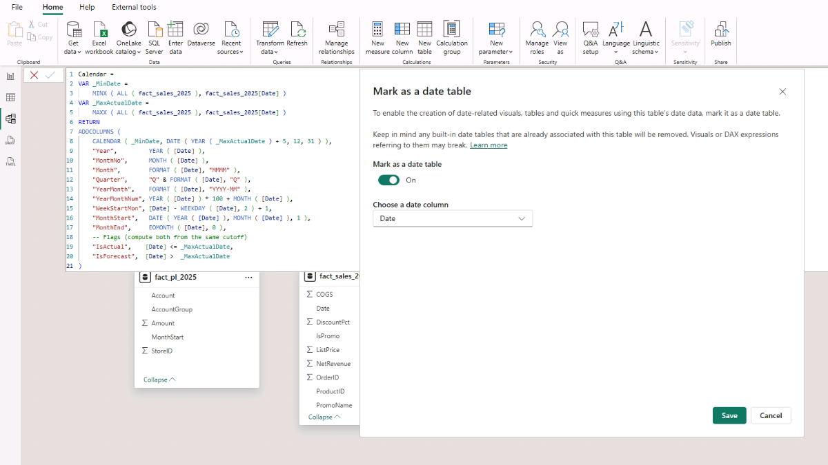
Once the table is created, right-click it and choose Mark as date table, then select the Date column. This tells Microsoft Power BI to use this table for all time-intelligence calculations.

With our calendar table ready, we can begin establishing relationships and building the data model.

Step 3. Building a Data Model in Microsoft Power BI

Now that our tables are loaded, let’s shape a tidy model that’s easy to slice, filter, and extend. We’ll create two small dimensions—DimCategory and DimSubcategory—directly from the product master, then connect everything into a classic star-style schema so filters flow from dimensions into facts.

Step 3a. Create Category and Subcategory Dimensions

Category and subcategory already live inside dim_products, so there’s no need for extra files. Let’s create two DAX tables to extract unique lists we can use for filtering and hierarchies.

Go to Model view and select New table. Paste the DAX for DimCategory:

DimCategory =
DISTINCT (
    SELECTCOLUMNS (
        dim_products,
        "Category", dim_products[Category]
    )
)

Then create DimSubcategory:

DimSubcategory =
DISTINCT (
    SELECTCOLUMNS (
        dim_products,
        "Subcategory", dim_products[Subcategory],
        "Category",    dim_products[Category]
    )
)

Why this works (brief DAX context): SELECTCOLUMNS() projects only the fields we need into a new table, and DISTINCT() ensures we get a clean, duplicate-free list—perfect for dimension tables and slicers.

Let’s link them so filters cascade appropriately: connect DimCategory[Category] → DimSubcategory[Category], then DimSubcategory[Subcategory] → dim_products[Subcategory]. Keep relationships one-to-many and single-direction (from dimension to fact). This gives us a neat Category → Subcategory → Product path that will drive our sales, margin, and forecast visuals.

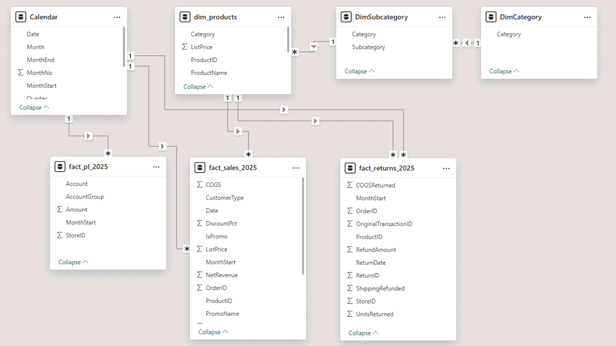
Step 3b. Finalize Model Relationships

Arrange dimensions across the top and fact tables underneath to make the lineage obvious. Then create these relationships:

• Calendar[Date] → fact_sales_2025[Date]
• Calendar[Date] → fact_returns_2025[ReturnDate]
• Calendar[Date] → fact_pl_2025[MonthStart]
• DimSubcategory[Subcategory] → dim_products[Subcategory]
• dim_products[ProductID] → fact_sales_2025[ProductID]
• dim_products[ProductID] → fact_returns_2025[ProductID]

Keep all relationships one-to-many and single-direction (dimension → fact). This creates a clean, intuitive star-style model, with one small snowflake exception for product categories, and gives predictable results with filters, time intelligence, and the DAX measures we’ll write next.

With the structure in place, we’re ready to introduce our first measures and start building the sales analysis.

Step 4. Monthly Sales Analysis with DAX Measures

Now that our model is wired up, let’s add the measures that power our sales revenue analysis in Microsoft Power BI. We’ll start with core totals and then introduce KPIs that explain pricing, basket size, returns, and profitability month by month.

To keep everything tidy, let’s create a dedicated table to hold our measures: Go to Home → Enter data, name it Measures_Table, and click Load. Then right-click the table and choose New measure

Step 4a. Base DAX Measures — Sales, Returns, COGS & Margin

These measures build the foundation of our reporting — giving us counts, revenue, costs, and profit to feed our dashboards and charts.

Orders, Transactions & Units – these counts tell us how many orders we processed, how many transaction lines they contained, and how many total units we sold — the essential volume drivers for our analysis.

-- Core counts
Orders =
DISTINCTCOUNT ( fact_sales_2025[OrderID] )

Transactions =
COUNTROWS ( fact_sales_2025 )

Units =
SUM ( fact_sales_2025[Units] )

Gross Sales, Net Revenue & Discounts – calculate list-price sales, the realized revenue after discounts, and the discount impact to analyze customer purchase patterns and promotional behavior over time.

-- Revenue & Discounts
Gross Sales (List Price) =
SUMX ( fact_sales_2025, fact_sales_2025[Units] * fact_sales_2025[ListPrice] )

Sales Revenue (After Discount, Before Returns) =
SUM ( fact_sales_2025[NetRevenue] )

Discount Amount =
- ( [Gross Sales (List Price)] - [Sales Revenue (After Discount, Before Returns)] )

Returns — Units & Value – these measures track how many items customers returned and the refunded value.

-- Returns (amount & units)
Returns Amount =
- SUM ( fact_returns_2025[RefundAmount] )

Units Returned =
SUM ( fact_returns_2025[UnitsReturned] )

Net Sales – combines revenue after discount with the impact of returns to give us true top-line performance.

-- Net Sales (after returns)
Net Sales =
[Sales Revenue (After Discount, Before Returns)] + [Returns Amount]

Cost of Goods Sold (COGS) – shown as negative (a cost). Returns reduce cost, so we add them back to reflect net cost.

-- COGS (costs negative; returns reduce cost)
COGS (Sales) =
- SUM ( fact_sales_2025[COGS] )

COGS (Returns) =
SUM ( fact_returns_2025[COGSReturned] )

COGS (Net) =
[COGS (Sales)] + [COGS (Returns)]

Shipping Cost – a company expense for both outbound orders and inbound returns, so both legs are treated as costs.

-- Shipping (both legs are company costs → negative)
Shipping (Sales) =
- SUM ( fact_sales_2025[ShippingCost] )

Shipping (Returns) =
- SUM ( fact_returns_2025[ShippingCost] )

Shipping (Total) =
[Shipping (Sales)] + [Shipping (Returns)]

Gross Margin & Operating Profit DAX – bring revenue and cost components together to calculate gross margin and, after OPEX, operating profit.

-- Profit ladders
Gross Margin ($) = 
[Net Sales] + [COGS (Net)] + [Shipping (Total)]

OPEX (Excl Shipping) (Actual) =
[Payroll (Actual)] + [Other OPEX (Actual)]

Operating Profit ($) =
[Gross Margin ($)] + [OPEX (Excl Shipping) (Actual)]

Step 4b. KPI DAX Measures — Pricing, Basket, Returns & Profitability

These KPIs turn raw totals into decision-ready signals: how customers buy, how much we discount, how returns trend, and where margins land as a share of sales.

Basket & Pricing – show how much customers spend per order and per item, and the profit contributed per unit.

-- Basket & pricing
Average Order Value (AOV) =
DIVIDE ( [Net Sales], [Orders] )

Items per Order =
DIVIDE ( [Units], [Orders] )

Average Selling Price (ASP) =
DIVIDE ( [Net Sales], [Units] )

Average COGS per Item =
DIVIDE ( - [COGS (Net)], [Units] )

Gross Margin per Item =
DIVIDE ( [Gross Margin ($)], [Units] )

Discount Performance DAX – tracks how much revenue we give away through discounts and promotions.

-- Discounts (positive %)
Effective Discount % =
DIVIDE ( - [Discount Amount], [Gross Sales (List Price)] )

Return Rates – capture product returns by volume and by revenue impact so we can monitor product quality and customer satisfaction.

-- Returns
Return Rate (Units) =
DIVIDE ( [Units Returned], [Units] )

Return Rate (Revenue) =
DIVIDE ( - [Returns Amount], [Sales Revenue (After Discount, Before Returns)] )

Margin & Cost Ratios – show profitability and the cost structure behind each unit of sales.

-- Margins (positive %)
Gross Margin % =
DIVIDE ( [Gross Margin ($)], [Net Sales] )

Operating Profit % = 
DIVIDE ( [Operating Profit ($)], [Net Sales] )

-- Cost ratios (use minus to invert negative totals)
COGS % of Sales =
DIVIDE ( - [COGS (Net)], [Net Sales] )

Average Shipping Cost per Order = 
DIVIDE ( - [Shipping (Total)], [Orders] )

Average Shipping Cost per Item = 
DIVIDE ( - [Shipping (Total)], [Units] )

Shipping % of Sales =
DIVIDE ( - [Shipping (Total)], [Net Sales] )

With our core measures and KPIs in place, we’re ready to bring the numbers to life. Next, we’ll design the monthly sales and margin dashboard so viewers can explore performance by month, category, and subcategory.

Step 5. Building the Monthly Sales Analysis in Microsoft Power BI

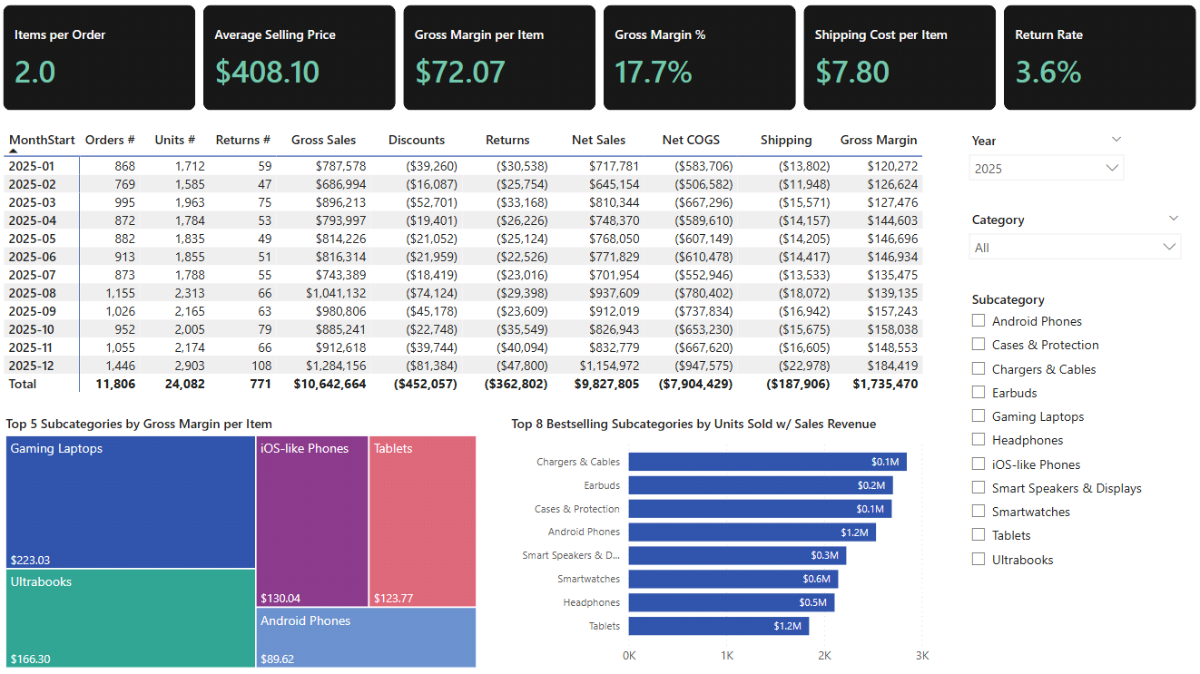
Let’s turn our measures into a clear monthly view that users can read in seconds. We’ll keep the page focused on actuals, use a matrix for monthly totals, and surface KPIs with cards. Then we’ll add two visuals to highlight margin and sales mix.

Step 5a. Analyze Monthly Totals and Surface the KPIs

Rename the page to something clear like Sales analysis. In the Filters on this page, set Calendar[IsActual] = True so the view focuses on historical performance.

Insert a Matrix visual. Add Calendar[MonthStart] to Rows, then format the field as yyyy-mm in the Format pane so months sort chronologically. Add our total measures to Values: Orders, Units, Units Returned, Gross Sales (List Price), Discount Amount, Returns Amount, Net Sales, COGS (Net), Shipping (Total), Gross Margin ($). Format money as currency and counts as whole numbers. If needed, use Rename for this visual to shorten column labels so the matrix remains readable.

Add slicers so readers can focus the story. Insert three Slicer visuals: Category (Dropdown), Subcategory (List), and Year (Dropdown). As expected, the Subcategory slicer will react to Category selection.

To change the slicer style (for example, switching between a dropdown and a vertical list), go to the slicer’s Format pane and select the layout you want in the Options section.

Finally, insert Card (new) visuals to display headline KPIs. Add Items per Order, Average Selling Price (ASP), Gross Margin per Item, Gross Margin %, Average Shipping Cost per Item, Return Rate (Revenue) — the set that best explains price, basket size, margin, and returns at a glance.

Step 5b. Analyze Gross Margin and Sales with Power BI Visuals

Add a Treemap to spotlight the biggest contributors by subcategory. Put Gross Margin per Item in Values and DimSubcategory[Subcategory] in Category. To keep the chart focused, open the Filters pane for this visual, switch to Top N, set Show items to Top 5, and use Gross Margin per Item as the By value. Turn on Data labels so the amounts are visible.

Next, add a Clustered bar chart to show the top sellers by units. Put DimSubcategory[Subcategory] on the Y-axis and Units on the X-axis. In the visual-level filters, set Subcategory → Top N → Top 8 by Units. Turn on Data labels, expand the options, and show Gross Sales (List Price) on the labels to pair volume with revenue. Adjust Display units, Decimal places, and label Position so the chart reads cleanly.

To stop the Subcategory slicer from over-filtering the charts, open Format → Edit interactions with the Subcategory slicer selected and set both charts to None. This keeps the charts stable while the matrix and cards remain fully interactive.

With the monthly dashboard in place, we’re ready to extend the model with parameters and build our interactive sales revenue forecast next.

Step 6. Monthly and Annual Retail Sales Forecast DAX Measures

We’re going to add a simple driver-based forecast on top of our actuals. We’ll control the forecast with parameters (percentage adjustments), and then reference prior-year results to project forward. The goal is an intuitive sales revenue forecast in Microsoft Power BI that reacts instantly when we adjust assumptions.

Step 6a. Power BI Parameters for Sales Forecast

Let’s create the parameters that will drive our scenario adjustments. Go to the Report View, then Modeling tab → New parameter → Numeric range and name the first parameter (for example, Items Sold). Use Decimal number as the data type and set the bounds so we can model decreases and increases.

Uncheck Add slicer to this page for now — we’ll place slicers later when we build the forecast report page.

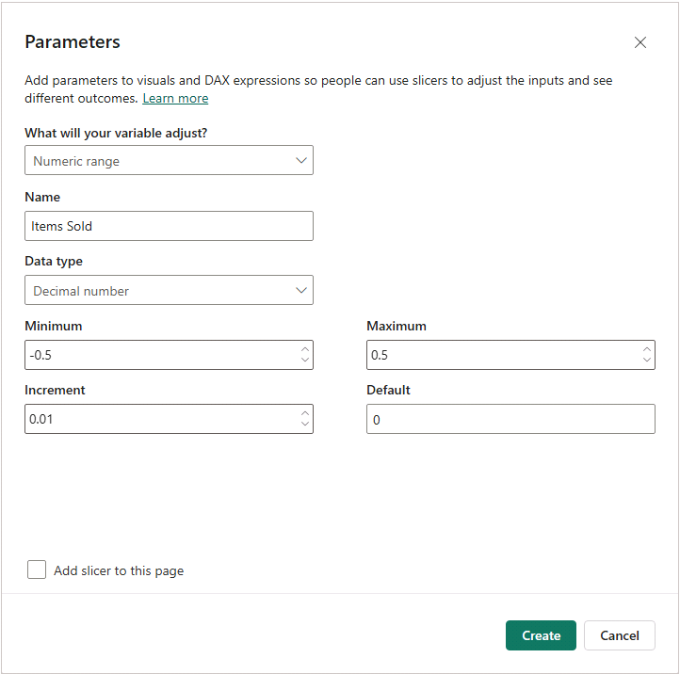
For this tutorial, set up the following parameters (all decimals with min -0.5, max 0.5, Increment 0.01, Default 0):

• Items Sold
• Average Selling Price
• COGS
• Shipping Cost
• Return Rate
• OPEX Salaries

These controls will let us nudge volumes, pricing, costs, and returns up or down and immediately see the impact on revenue, gross margin, and operating profit.

Step 6b. DAX Measures for the Retail Sales Forecast

Below we’ll introduce small helper measures and then define the forecasted totals by referencing prior-year values and applying our parameter multipliers combined with Power BI’s DATEADD function (external link).

Parameter Multipliers – convert each parameter slider into a multiplier we can apply repeatedly year over year.

-- Parameter Multipliers
Items Sold Multiplier =
1 + 'Items Sold'[Items Sold Value]

Average Selling Price Multiplier =
1 + 'Average Selling Price'[Average Selling Price Value]

COGS Multiplier =
1 + 'COGS'[COGS Value]

Shipping Cost Multiplier =
1 + 'Shipping Cost'[Shipping Cost Value]

Return Rate Multiplier =
1 + 'Return Rate'[Return Rate Value]

OPEX Salaries Multiplier =
1 + 'OPEX Salaries'[OPEX Salaries Value]

Tiny helpers (scalar, no recursion) – find the last actual date in our dataset and calculate how many years ahead the current context is, so we only show forecasted values in future periods.

-- Tiny helpers (scalar, no recursion)
Max Actual Date =
CALCULATE ( MAX ( fact_sales_2025[Date] ), ALL ( fact_sales_2025 ) )

Max Actual Year =
YEAR ( [Max Actual Date] )

Years Ahead =
VAR _y = YEAR ( MAX ( Calendar[Date] ) )
RETURN MAX ( 0, _y - [Max Actual Year] )

Note: Years Ahead measure returns 0 for actuals (so forecast measures return BLANK there), 1 for the first forecast year, 2 for the second, and so on.

Orders & Units (Forecast) – project order counts and units by taking the prior year as a base and applying the Items Sold multiplier.

-- Orders & Units
Orders (Forecast) =
VAR n = [Years Ahead]
RETURN
IF (
    n = 0,
    BLANK(),
    VAR Base =
        CALCULATE ( [Orders], DATEADD ( Calendar[Date], -n, YEAR ) )
    RETURN Base * POWER ( [Items Sold Multiplier], n )
)

Units (Forecast) =
VAR n = [Years Ahead]
RETURN
IF (
    n = 0,
    BLANK(),
    VAR Base =
        CALCULATE ( [Units], DATEADD ( Calendar[Date], -n, YEAR ) )
    RETURN Base * POWER ( [Items Sold Multiplier], n )
)

Revenue & Returns (Forecast) – extends revenue by applying both volume and price multipliers, and adjusts returns by volume, price, and return-rate multipliers.

-- Revenue & Returns
Gross Sales (List Price) (Forecast) =
VAR n = [Years Ahead]
RETURN
IF (
    n = 0,
    BLANK(),
    VAR Base =
        CALCULATE ( [Gross Sales (List Price)], DATEADD ( Calendar[Date], -n, YEAR ) )
    RETURN
        Base
        * POWER ( [Items Sold Multiplier], n )
        * POWER ( [Average Selling Price Multiplier], n )
)

Sales Revenue (Before Returns) (Forecast) =
VAR n = [Years Ahead]
RETURN
IF (
    n = 0,
    BLANK(),
    VAR Base =
        CALCULATE ( [Sales Revenue (After Discount, Before Returns)], DATEADD ( Calendar[Date], -n, YEAR ) )
    RETURN Base
        * POWER ( [Items Sold Multiplier], n )
        * POWER ( [Average Selling Price Multiplier], n )
)

Returns Amount (Forecast) =
VAR n = [Years Ahead]
RETURN
IF (
    n = 0,
    BLANK(),
    VAR Base =
        CALCULATE ( [Returns Amount], DATEADD ( Calendar[Date], -n, YEAR ) )
    RETURN Base
        * POWER ( [Items Sold Multiplier], n )
        * POWER ( [Average Selling Price Multiplier], n )
        * POWER ( [Return Rate Multiplier], n )
)

Units Returned (Forecast) =
VAR n = [Years Ahead]
RETURN
IF (
    n = 0,
    BLANK(),
    VAR Base =
        CALCULATE ( [Units Returned], DATEADD ( Calendar[Date], -n, YEAR ) )
    RETURN Base
        * POWER ( [Items Sold Multiplier], n )
        * POWER ( [Return Rate Multiplier], n )
)

Net Sales (Forecast) =
[Sales Revenue (Before Returns) (Forecast)] + [Returns Amount (Forecast)]

COGS (Forecast) – project cost of goods proportionally with volumes and the COGS multiplier; returns reduce cost as before.

-- COGS
COGS (Sales) (Forecast) =
VAR n = [Years Ahead]
RETURN
IF (
    n = 0,
    BLANK(),
    VAR Base =
        CALCULATE ( [COGS (Sales)], DATEADD ( Calendar[Date], -n, YEAR ) )
    RETURN Base
        * POWER ( [Items Sold Multiplier], n )
        * POWER ( [COGS Multiplier], n )
)

-- Positive reduction to cost
COGS (Returns) (Forecast) =
VAR n = [Years Ahead]
RETURN
IF (
    n = 0,
    BLANK(),
    VAR Base =
        CALCULATE ( [COGS (Returns)], DATEADD ( Calendar[Date], -n, YEAR ) )
    RETURN Base
        * POWER ( [Items Sold Multiplier], n )
        * POWER ( [Return Rate Multiplier], n )
        * POWER ( [COGS Multiplier], n )
)

COGS (Net) (Forecast) =
[COGS (Sales) (Forecast)] + [COGS (Returns) (Forecast)]

Shipping (Forecast) – forecast outbound and returns shipping as costs influenced by volume, return rate, and shipping cost assumptions.

-- Shipping
Shipping (Sales) (Forecast) =
VAR n = [Years Ahead]
RETURN
IF (
    n = 0,
    BLANK(),
    VAR Base =
        CALCULATE ( [Shipping (Sales)], DATEADD ( Calendar[Date], -n, YEAR ) )
    RETURN Base
        * POWER ( [Items Sold Multiplier], n )
        * POWER ( [Shipping Cost Multiplier], n )
)

Shipping (Returns) (Forecast) =
VAR n = [Years Ahead]
RETURN
IF (
    n = 0,
    BLANK(),
    VAR Base =
        CALCULATE ( [Shipping (Returns)], DATEADD ( Calendar[Date], -n, YEAR ) )
    RETURN Base
        * POWER ( [Items Sold Multiplier], n )
        * POWER ( [Return Rate Multiplier], n )
        * POWER ( [Shipping Cost Multiplier], n )
)

Shipping (Total) (Forecast) =
[Shipping (Sales) (Forecast)] + [Shipping (Returns) (Forecast)]

Gross Margin (Forecast) – combines forecasted sales, COGS, and shipping to produce gross margin — consistent with the sign conventions we used for actuals.

-- Gross Margin (includes shipping, per your convention)
Gross Margin ($) (Forecast) =
[Net Sales (Forecast)]
+ [COGS (Net) (Forecast)]
+ [Shipping (Total) (Forecast)]

OPEX & Operating Profit (Forecast) – project payroll and other OPEX using the same compounding idea, then calculates operating profit from forecasted gross margin and OPEX.

-- OPEX (excl. shipping), using same compounding idea
Payroll (Actual) =
CALCULATE (
    SUM ( fact_pl_2025[Amount] ),
    fact_pl_2025[Account] = "Payroll (incl. taxes & bonus)"
)

Other OPEX (Actual) =
CALCULATE (
    SUM ( fact_pl_2025[Amount] ),
    fact_pl_2025[AccountGroup] = "OPEX",
    fact_pl_2025[Account] <> "Payroll (incl. taxes & bonus)",
    fact_pl_2025[Account] <> "Logistics / Shipping"
)

Payroll (Forecast) =
VAR n = [Years Ahead]
RETURN
IF (
    n = 0,
    BLANK(),
    VAR Base =
        CALCULATE ( [Payroll (Actual)], DATEADD ( Calendar[Date], -n, YEAR ) )
    RETURN Base * POWER ( [OPEX Salaries Multiplier], n )
)

Other OPEX (Forecast) =
VAR n = [Years Ahead]
RETURN
IF (
    n = 0,
    BLANK(),
    VAR Base =
        CALCULATE ( [Other OPEX (Actual)], DATEADD ( Calendar[Date], -n, YEAR ) )
    RETURN Base * POWER ( [OPEX Salaries Multiplier], n )
)

OPEX (Excl Shipping) (Forecast) =
[Payroll (Forecast)] + [Other OPEX (Forecast)]

Operating Profit ($) (Forecast) =
[Gross Margin ($) (Forecast)] + [OPEX (Excl Shipping) (Forecast)]

These measures give us a driver-based forecast that scales with simple business assumptions. In the next step, we’ll turn these into an interactive page where we can adjust parameters and immediately see their effect on units, sales revenue, costs, and profitability.

Step 7. Building an Interactive Forecast Dashboard in Microsoft Power BI

Let’s bring the forecast to life. We’ll add slicers for our parameters, build a simple year-by-year matrix that shows forecast values alongside prior-year comparisons, and apply conditional formatting so wins and risks pop immediately.

Step 7a. Add Parameter Slicers and Set Their Behavior

Insert a Slicer visual and add ‘Items Sold’[Items Sold]. In the Slicer header, give it a clear title like Items Sold Adjustment (%). In Slicer settings, choose Single value and turn on the Slider. Format the field as a percentage so it reads naturally. Repeat the same steps for Average Selling Price, COGS, Shipping Cost, Return Rate, and OPEX Salaries.

Step 7b. Build the Year Matrix and Place the Forecast DAX Measures

Insert a Matrix and add Calendar[Year] to Rows. For Values, start with: Units (Forecast), Net Sales (Forecast), COGS (Net) (Forecast), Shipping (Total) (Forecast), Gross Margin ($) (Forecast), Payroll (Forecast), Other OPEX (Forecast), Operating Profit ($) (Forecast). Keep money as currency and counts as whole numbers.

Now add the variance measures near each base value so year-on-year dynamics are obvious. Paste each measure as its own code block.

Units Var – absolute change in units versus prior year.

Units Var =
IF (
    [Years Ahead] = 0,
    BLANK(),
    VAR Prior =
        COALESCE(
            CALCULATE ( [Units (Forecast)], DATEADD ( Calendar[Date], -1, YEAR ) ),
            CALCULATE ( [Units],            DATEADD ( Calendar[Date], -1, YEAR ) )
        )
    RETURN
        [Units (Forecast)] - Prior
)

Net Sales Var (%) -percent change in net sales versus prior year.

Net Sales Var (%) =
IF (
    [Years Ahead] = 0,
    BLANK(),
    VAR Prior =
        COALESCE(
            CALCULATE ( [Net Sales (Forecast)], DATEADD ( Calendar[Date], -1, YEAR ) ),
            CALCULATE ( [Net Sales],            DATEADD ( Calendar[Date], -1, YEAR ) )
        )
    RETURN
        DIVIDE ( [Net Sales Var ($)], Prior )
)

COGS (Net) Var (%) – percent change in net COGS versus prior year.

COGS (Net) Var (%) =
IF (
    [Years Ahead] = 0,
    BLANK(),
    VAR Prior =
        COALESCE(
            CALCULATE ( [COGS (Net) (Forecast)], DATEADD ( Calendar[Date], -1, YEAR ) ),
            CALCULATE ( [COGS (Net)],            DATEADD ( Calendar[Date], -1, YEAR ) )
        )
    RETURN
        DIVIDE ( [COGS (Net) Var ($)], Prior )
)

Shipping (Total) Var ($) – absolute change in total shipping cost.

Shipping (Total) Var ($) =
IF (
    [Years Ahead] = 0,
    BLANK(),
    VAR Prior =
        COALESCE(
            CALCULATE ( [Shipping (Total) (Forecast)], DATEADD ( Calendar[Date], -1, YEAR ) ),
            CALCULATE ( [Shipping (Total)],            DATEADD ( Calendar[Date], -1, YEAR ) )
        )
    RETURN
        [Shipping (Total) (Forecast)] - Prior
)

Gross Margin Var (%) – percent change in gross margin dollars.

Gross Margin Var (%) =
IF (
    [Years Ahead] = 0,
    BLANK(),
    VAR Prior =
        COALESCE(
            CALCULATE ( [Gross Margin ($) (Forecast)], DATEADD ( Calendar[Date], -1, YEAR ) ),
            CALCULATE ( [Gross Margin ($)],            DATEADD ( Calendar[Date], -1, YEAR ) )
        )
    RETURN
        DIVIDE ( [Gross Margin ($) Var], Prior )
)

Gross Margin Var (%pp) – change in gross margin rate in percentage points.

Gross Margin Var (%pp) = 
IF (
    [Years Ahead] = 0,
    BLANK(),
    VAR PriorRate =
        COALESCE(
            CALCULATE ( [Gross Margin % (Forecast)], DATEADD ( Calendar[Date], -1, YEAR ) ),
            CALCULATE ( [Gross Margin %],            DATEADD ( Calendar[Date], -1, YEAR ) )
        )
    RETURN
        [Gross Margin % (Forecast)] - PriorRate
)

Step 7c. Completing the Sales Forecast Dashboard

Now add the two rate measures to the Power BI matrix, which will complete the picture.

Gross Margin % (Forecast)

Gross Margin % (Forecast) =
DIVIDE ( [Gross Margin ($) (Forecast)], [Net Sales (Forecast)] )

Operating Profit % (Forecast)

Operating Profit % (Forecast) = 
DIVIDE ( [Operating Profit ($) (Forecast)], [Net Sales (Forecast)] )

Apply conditional formatting so variances read at a glance. In the Format pane → Cell elements, select each variance series (for example, Units Var), turn on Font color, and use the fx button to configure rules.

Set negative values using ≥ Min and < 0, and positive values using > 0 and ≤ Max. Repeat for the other variance and KPI measures.

If labels feel long, use Rename for this visual to shorten them without changing the underlying measure names.

Add a final Category slicer (Dropdown) to filter the forecast by product category.

To visualize the forecast month by month, add a Line and clustered column chart. Put Calendar[MonthStart] on X-axis, Net Sales (Forecast) on Column y-axis, and Units (Forecast) on Line y-axis. This gives a quick view of seasonality and how volume and revenue move together under different parameter settings.

Step 8. Scenario & What-If Analysis in Microsoft Power BI

With the forecast dashboard in place, let’s stress-test our model using the preview below. We’ll adjust the parameter slicers to see how small changes in volume, pricing, costs, and returns flow through net sales, gross margin, and operating profit. The point is not to predict the future perfectly, but to understand sensitivity and risk.

Baseline (Status Quo)

• Set all parameters to 0% (Items Sold, Average Selling Price, COGS, Shipping Cost, Return Rate).
• This anchors the story: forecast periods (2026+) mirror 2025 actuals.
• Use it as the reference state before exploring alternatives.

Healthy Growth with Stable Margins (Scenario 1)

• Try Items Sold +10%, Average Selling Price +3%, COGS +3%, Shipping Cost +2%, Return Rate 0%.
• Orders and revenue increase primarily from volume, with a small price lift. Costs scale proportionally, keeping Gross Margin % roughly steady while Gross Margin $ rises ~10–13%.
• This is a clean illustration of steady expansion without margin erosion.

Price Inflation vs Cost Pressure (Scenario 2)

• Set Average Selling Price +5%, COGS +7%, Shipping Cost +5%, with Items Sold 0% and Return Rate 0%.
• Revenue grows on price, but costs grow faster. Expect Net Sales up ~5%, Gross Margin $ up only ~1–2%, and Gross Margin % lower by roughly 1–2 pp.
• This shows how inflation can erode profitability even when top-line looks healthy.

Aggressive Volume Growth & Operational Stress (Scenario 3)

• Set Items Sold +20%, Average Selling Price 0%, COGS +3%, Shipping Cost +5%, Return Rate +2%.
• Revenue and orders jump on volume, but higher logistics costs and a rising return rate trim efficiency.
• You’ll see a strong increase in Net Sales with a slight decline in Gross Margin % — a useful illustration of the scale vs. cost-control trade-off.

As you move the sliders, watch three places: the year matrix (volume, revenue, and profit by year), the variance fields (what’s changing vs. prior year), and the monthly chart for seasonality under different assumptions.

📌 Recap: Building a Sales Analysis & Forecast Model in Microsoft Power BI

Here’s a quick recap of the steps we followed to build a complete sales analysis and revenue forecast model in Microsoft Power BI:

1. Load and explore sales data. We imported sales, returns, product master data, and a monthly P&L, then previewed each table to understand how orders, returns, and costs behave across the year.
2. Create a dynamic calendar table. We built a DAX-powered Calendar table that runs from first sale through five future years, then marked it as the official date table to enable time intelligence.
3. Model data into a star-style schema. We created Category and Subcategory dimensions, linked products to sales and returns, and connected everything to Calendar for a clean, scalable reporting model.
4. Build foundational sales & margin measures. We defined core metrics such as Orders, Units, Net Sales, COGS, Shipping, and Gross Margin — the foundation of retail analytics.
5. Surface retail KPIs. We added essential commercial performance measures: AOV, Items per Order, Gross Margin %, Shipping Cost per Item, and Return Rates to reveal pricing, basket behavior, and product efficiency.
6. Build the monthly sales analysis dashboard. We combined a monthly matrix, slicers, KPI cards, and visuals like a treemap and top-product chart to explore seasonality and product profitability.
7. Add scenario drivers & forecast DAX. We created what-if parameters (Items Sold, Price, COGS, Shipping, Return Rate, OPEX) and a full parallel set of forecast measures using compound growth logic.
8. Build the forecast & sensitivity view. We added forecast matrix visuals, YoY variance fields, conditional formatting, and a monthly forecast chart to test volume, price, and cost scenarios.

By following these steps, you now have a Power BI model that analyzes sales performance, evaluates profitability, and forecasts future revenue under different business assumptions.

🔎 Preview the Interactive Sales Analysis & Forecast Dashboard

Explore the finished sales analysis and forecasting dashboard — the same build from this tutorial. Adjust parameters and see how changes in volume, pricing, COGS, and return rates impact sales and profitability.

📥 Download My Sales Analysis & Forecast Dashboard Template

To help you get started quickly, I’ve prepared a ready-to-use Power BI package that includes:

• Power BI (.pbix) file with all sales and forecast logic, parameters, and dashboards.
• CSV files for sales, returns, products, and P&L so you can explore the data model end-to-end.
• Text file with all DAX measures fully organized for easy reference.

This package lets you analyze sales performance, identify key revenue drivers, and test growth scenarios.

👁️ View full template details

Get in Touch

Hi, I’m Jacek. I’m passionate about Microsoft Power BI, DAX, and analytics. I hope this tutorial helped you explore sales performance, build interactive dashboards, and forecast revenue with dynamic assumptions.

If you’d like guidance on analytics, pricing models, or commercial forecasting, feel free to get in touch.

You can also explore my other tutorials for more step-by-step guides, or check out my One-to-One Training and Data Analytics Support if you’d like personalized help.

Disclaimer: This tutorial is for informational and educational purposes only and should not be considered professional advice.

Explore More Tutorials

• • Power BI Financial Planning & Analysis Dashboard Tutorial — Build a fully integrated FP&A dashboard, combining P&L, cash flow, balance sheet, and forecasting logic.
  • Power BI Consolidated P&L Forecast Tutorial — Build a multi-entity profit & loss forecast in Microsoft Power BI using clean DAX measures and a robust star schema.
  • Excel Cash Flow Forecast Tutorial — Create a dynamic 3-statement cash flow model to plan liquidity and visualize inflows and outflows over time.
  • Excel Monthly Budget & Forecast Tutorial — Build a monthly budgeting and variance tracker with rolling forecasts and clear management reporting.
  • Power BI Marketing Performance & Forecast Dashboard — Track campaigns, CAC, ROAS, and forecast marketing outcomes with interactive visuals in Microsoft Power BI.